The machine-learning model featured in my previous post was a regression model that predicted taxi fares based on distance traveled, the day of the week, and the time of day. Now it’s time to tackle classification models, which predict categorical outcomes such as what type of flower a set of measurements represent or whether a credit-card transaction is fraudulent.
Recall that classification models fall into two categories: binary-classification models, in which there are just two possible outcomes, and multiclass-classification models, in which there are more than two possible outcomes. You have already seen one example of multiclass classification in this series, and you will see more. But for now, let’s dive into binary classification, starting with the go-to learning algorithm that data scientists use more often than any other for binary-classification problems.
Logistic Regression
There are many learning algorithms that can be used for binary classification. In my post on regression algorithms, you learned how decision trees, random forests, and gradient-boosting machines can be used for regression models. These algorithms can be used for classification as well, and Scikit helps out by offering classes such as DecisionTreeClassifier, RandomForestClassifier, and GradientBoostingClassifier. In my post on supervised learning, you saw k-nearest neighbors and Scikit’s KNeighborsClassifier class used to build a 3-class classification model.
These are important learning algorithms, and they see use in many contemporary machine-learning models. But one of the most popular classification algorithms of all is logistic regression, which looks at a distribution of data and fits an equation to it that defines the probability that a given sample belongs to each of two possible classes. It might determine, for example, that there’s a 10% chance that the values in a given row correspond to class 0 and a 90% chance that they correspond to class 1. In this case, logistic regression will predict that the sample corresponds to class 1. Despite the name, logistic regression is a classification algorithm, not a regression algorithm. Its purpose is not to create regression models. It is to quantify probabilities for the purpose of performing binary classification.
As an example, consider the data points below, which belong to two classes: 0 (blue) and 1 (red). The blues fall in the range x=0 to x=10, while the reds fall in the range x=5 to x=15. You can’t pick a value for x that separates the classes since both have values between x=5 and x=10. (Try drawing a vertical line that has only reds on one side and only blues on the other.) But you can draw a curve that, given an x, shows the probability that a point with that x belongs to class 1. As x increases, so too does the likelihood that the point represents class 1 rather than class 0. From the curve, you can see that if x=2, there is less than a 5% chance that the point corresponds to class 1. But if x=10, there is about a 76% chance that it’s class 1. If asked to classify that point as a red or a blue, we would conclude that it’s a red because it’s much more likely to be red than blue.
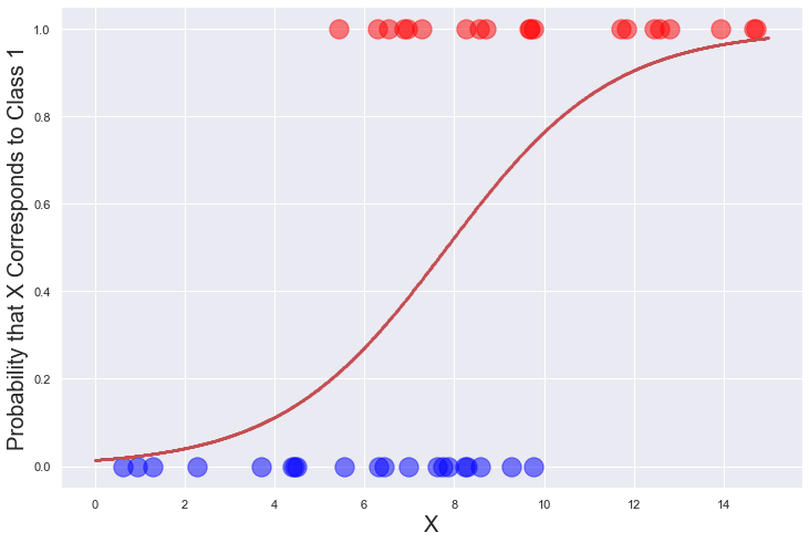
The curve in the diagram above is a sigmoid curve. It charts a function known as the logistic function (also known as the logit function) that has been used in statistics for decades, and from which logistic regression takes its name. For logistic regression, the logistic function is defined this way, where x is the input value and m and b are parameters that are learned during training:
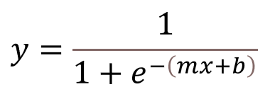
The logistic-regression learning algorithm fits the logistic function to a distribution of data and uses the resulting y values as probabilities in order to classify data points. It works with any number of features (not just x, but x1, x2, x3, and so on), and it is a parametric learning algorithm since it uses the training data to find optimum values for m and b. How it finds the optimum values is an implementational detail that libraries such as Scikit-learn handle for you. Scikit defaults to a numerical optimization algorithm known as Limited-memory Broyden–Fletcher–Goldfarb–Shanno (L-BFGS) but supports other optimization methods as well. This, incidentally, is one reason why Scikit is so popular in the machine-learning community. It’s not difficult to calculate m and b from the training data for a linear-regression model, but it is much harder to do it for a logistic-regression model, not to mention more sophisticated parametric models such as support-vector machines.
Scikit’s LogisticRegression class is logistic regression in a box. With it, training a logistic-regression model can be as simple as this:
model = LogisticRegression()
model.fit(x, y)
Once the model is trained, you can call its predict method to predict which class the input belongs (0 or 1), or its predict_proba method to get the computed probabilities. If you fit a LogisticRegression model to the dataset in the diagram above, the following statement predicts whether x=10 corresponds to class 0 or class 1:
predicted_class = model.predict([[10.0]])[0]
print(predicted_class) # Outputs 1
And these statements show the probabilities for each class that the model computed:
predicted_probabilties = model.predict_proba([[10.0]])[0]
print(f'Class 0: {predicted_probabilties[0]}') # 0.23508543966167028
print(f'Class 1: {predicted_probabilties[1]}') # 0.7649145603383297
Scikit also includes the LogisticRegressionCV class for training logistic-regression models with built-in cross-validation. Cross-validation was introduced in the previous post in this series. At the expense of additional training time, the following statements train a logistic-regression model using five folds:
model = LogisticRegressionCV(cv=5)
model.fit(x, y)
LogisticRegressionCV defaults to five folds in Scikit version 0.22 and higher, so you can omit the cv parameter if five folds are acceptable.
Logistic regression is technically a binary-classification algorithm, but it can be extended to perform multiclass classification, too. I’ll discuss this more in a future post on multiclass classification. For now, think of logistic regression as a machine-learning algorithm that uses the well-known logistic function to quantify the probability that an input corresponds to either of two classes and you have an accurate understanding of what logistic regression is.
Scoring Classification Models
You can quantify the accuracy of a classification model the same way you do for a regression model: by calling the model’s score method. For logistic regression, score returns the sum of the true positives and the true negatives divided by the total number of samples. If the test data includes 10 positives (samples of class 1) and 10 negatives (samples of class 0) and during testing the model identifies 8 of the positives correctly and 7 of the negatives, then the score is 8 + 7 / 20, or 0.75. This is sometimes referred to as the model’s accuracy score.
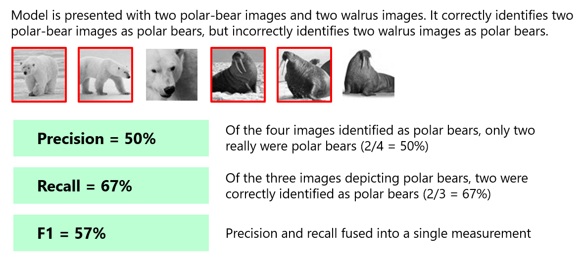
There are other ways to score a classification model, and which one is “right” often depends on how the model will be used. Rather than compute an accuracy score, data scientists sometimes measure a classification model’s precision or recall instead. Precision is computed by dividing the number of true positives by the sum of the true positives and false positives. Recall is computed by dividing the number of true positives by the sum of the true positives and false negatives.
The diagram below illustrates the difference. Suppose you train a model to differentiate between polar-bear images and walrus images, and to test it, you submit three polar-bear images and three walrus images. Furthermore, assume that the model correctly classifies two of the polar-bear images, but incorrectly classifies two walrus images as polar-bear images. In this case, the model’s precision in identifying polar bears is 50%, because only two of the four images the model classified as polar bears were in fact polar bears. But recall is 67% since the model correctly identified two of the three polar-bear images. That is precision and recall in a nutshell. The former quantifies the model’s ability to not label as positive a sample that is negative, while the latter quantifies the model’s ability to identify positive samples. The two can be combined into one score called the F1 score (or simply the F-score) using a simple formula.
Scikit provides helpful functions such as precision_score, recall_score, and f1_score for retrieving classification metrics for individual classes or for the model as a whole. Whether you prefer precision or recall depends on which is higher: the cost of false positives, or the cost of false negatives. Use precision when the cost of false positives is high — for example, when “positive” means a credit-card transaction is fraudulent. Credit-card companies would rather let 100 fraudulent transactions go through than suffer one false positive causing a legitimate transaction to be declined (and a customer to be angered.) By contrast, use recall if the cost of false negatives is high. A great example is when using machine learning to spot tumors in X-rays and MRIs. You would much rather erroneously send a patient to a doctor as a result of a false positive than tell that patient there are no tumors when there really are.
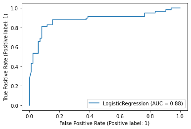
Accuracy score, precision, recall, and F1 score apply to binary-classification and multiclass-classification models. An additional metric — one that applies to binary classification only — is the receiver operating characteristic (ROC) curve, which plots the true-positive rate (TPR) against the false-positive rate (FPR) at various probability thresholds. A sample ROC curve is shown below. A straight line stretching from lower left to upper right would indicate that the model gets it right just 50% of the time. The more the curve arches toward the upper-left corner, the more accurate the model. In particular, data scientists often use the area under the curve (AUC, or ROC AUC) as a means for quantifying accuracy. Scikit provides a handy plot_roc_curve function for plotting an ROC curve, and a function named roc_auc_score for retrieving the ROC AUC score. The score returned by this function is a value between 0.0 and 1.0.
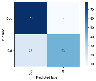
Yet another way to assess a classification model for accuracy is to plot a confusion matrix like the one pictured below. It works for binary and multiclass classification, and it shows for each class how the model performed during testing. In this example, the model was asked to differentiate between images containing dogs and images containing cats. It got it right 78 out of 85 times when presented with dog pictures, and 41 of 58 times when presented with cat pictures. Scikit offers a confusion_matrix function for computing a confusion matrix, and a plot_confusion_matrix function for plotting confusion matrices like the one below.
Categorical Data
Machine learning finds patterns in numbers. It only works with numbers. And yet many datasets have columns containing string values such as “male” and “female” or “red,” “green,” and “blue.” Data scientists refer to these as categorical values and the columns that contain them as categorical columns. Machine learning can’t handle categorical values directly. To use them in a model, you must convert them into numbers.
There are two popular algorithms for converting categorical values into numerical values. One is label encoding, which you briefly saw in the second post in this series. Label encoding replaces categorical values with integers. If there are three unique values in a column, label encoding replaces them with 0s, 1s, and 2s. To demonstrate, run the following code in a Jupyter notebook:
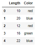
import pandas as pd
from sklearn.preprocessing import LabelEncoder

data = [[10, 'red'], [20, 'blue'], [12, 'red'], [16, 'green'], [22, 'blue']]
df = pd.DataFrame(data, columns=['Length', 'Color'])

encoder = LabelEncoder()
df['Color'] = encoder.fit_transform(df['Color'])
df.head()
This code creates a dataset containing a categorical column named “Color,” which contains three different categorical values. Here’s what the dataset looks like before encoding:
And here’s how it looks after the values in the “Color” column are label-encoded using Scikit’s LabelEncoder class:
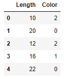
The encoded dataset can be used to train a machine-learning model. The unencoded dataset cannot. You can get an ordered list of the classes that were encoded from the encoder’s classes_ attribute.
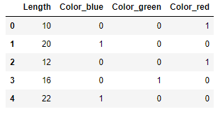
The other, more popular, means for converting categorical values into numeric values is one-hot encoding, which adds one column to the dataset for each unique value in a categorical column and fills the encoded columns with 1s and 0s. One-hot-encoding can be performed with Scikit’s OneHotEncoder class or by calling get_dummies on a Pandas DataFrame. Here is how the latter is used to encode the dataset:
data = [[10, 'red'], [20, 'blue'], [12, 'red'], [16, 'green'], [22, 'blue']]
df = pd.DataFrame(data, columns=['Length', 'Color'])

df = pd.get_dummies(df, columns=['Color'])
df.head()
And here are the results:
Label encoding and one-hot encoding are used with regression problems and classification problems. The obvious question is which one should you use? Generally speaking, data scientists prefer one-hot encoding to label encoding. The former gives every unique value an equal weight, whereas label encoding implies that some values may be more important than others – for example, that “red” (2) is more important than “blue” (0). The truth is that it often doesn’t matter. If in doubt, you rarely go wrong with one-hot encoding. And if you want to be certain, you can encode the data both ways and compare the results after using them to train a machine-learning model.
Classify Passengers Who Sailed on the Titanic
One of the more famous public datasets in machine learning is the Titanic dataset, which contains information regarding hundreds of passengers who sailed on the ill-fated voyage of the RMS Titanic, including which ones survived (and which ones did not). Let’s use logistic regression to build a binary-classification model from the dataset and see if we can predict the odds that a passenger will survive given the passenger’s gender, age, and fare class (whether they traveled in first, second, or third class).
The first step is to download the dataset and copy it to the “Data” subdirectory of the directory that hosts your Jupyter notebooks. Then run the following code in a notebook to load the dataset and get a feel for its contents:
import pandas as pd

df = pd.read_csv('Data/titanic.csv')
df.head()
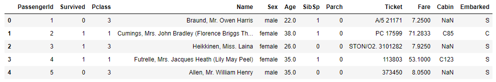
The dataset contains 891 rows and 12 columns. Some of the columns aren’t relevant to a machine-learning model, such as “PassengerId” and “Name.” Others are very relevant. The ones we’ll focus on are:
- Survived, which indicates whether the passenger survived the voyage (1) or did not (0)
- Pclass, which indicates whether the passenger was traveling in first class (1), second class (2), or third class (3)
- Sex, which indicates the passenger’s gender
- Age, which indicates the passenger’s age
The “Survived” column is the label column – the one we’ll try to predict. The other columns are relevant because first-class passengers were more likely to have survived the sinking, and women and children were more likely to be given space in lifeboats.
Now use the following statement to see if the dataset is missing any values:
df.info()
Here’s the output:
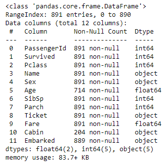
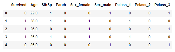
The “Cabin” column is missing a lot of values, but we don’t care since we’re not using that column. We are going to use the “Age” column, and that column is missing some values as well. We could replace the missing values with the mean of all the other ages, but we’ll take the simpler approach of removing rows with missing values. Use the following statements to remove the columns that we don’t need, drop rows with missing values, and one-hot-encode the values in the “Sex” and “Pclass” columns:
df = df[['Survived', 'Age', 'Sex', 'Pclass']]
df = pd.get_dummies(df, columns=['Sex', 'Pclass'])
df.dropna(inplace=True)
df.head()
Here is the resulting dataset:
The next task is to split the dataset for training and testing:
from sklearn.model_selection import train_test_split

x = df.drop('Survived', axis=1)
y = df['Survived']

x_train, x_test, y_train, y_test = train_test_split(x, y, test_size=0.2, stratify=y, random_state=0)
Note the stratify=y parameter passed to train_test_split. That’s important, because of the 714 samples remaining after rows with missing values are removed, 290 represent passengers who survived, and 424 represent passengers who did not. We want the training dataset and the test dataset to contain similar proportions of both classes, and stratify=y accomplishes that. Without stratification, the model might appear to be more or less accurate than it really is.
Now create a logistic-regression model, train it with the data split off for training, and score it with the test data:
from sklearn.linear_model import LogisticRegression

model = LogisticRegression(random_state=0)
model.fit(x_train, y_train)
model.score(x_test, y_test)
Score the model again using cross-validation so we have more confidence in the score:
from sklearn.model_selection import cross_val_score

cross_val_score(model, x, y, cv=5).mean()
Use the following statements to display a confusion matrix showing precisely how the model performed during testing:
%matplotlib inline
from sklearn.metrics import plot_confusion_matrix

plot_confusion_matrix(model, x_test, y_test, display_labels=['Perished', 'Survived'], cmap='Blues', xticks_rotation='vertical')
Finally, visualize the model’s accuracy by plotting an ROC curve:
from sklearn.metrics import plot_roc_curve

plot_roc_curve(model, x_test, y_test)
Now let’s use the trained model to make some predictions. First, let’s find out whether a 30-year female traveling in first class is likely to survive the voyage:
female = [[30, 1, 0, 1, 0, 0]]
model.predict(female)[0]
The model predicts that she will survive, but what are the odds that she we will survive?
probability = model.predict_proba(female)[0][1]
print(f'Probability of survival: {probability:.1%}')
A 30-year-old female traveling in first class is more than 90% likely to survive the voyage, but what about a 60-year-old male traveling in third class?
male = [[60, 0, 1, 0, 0, 1]]
probability = model.predict_proba(male)[0][1]
print(f'Probability of survival: {probability:.1%}')
Feel free to experiment with other inputs to see what the model says. How likely, for example, is a 12-year-old male traveling in second class to survive the sinking of the Titanic?
Get the Code
You can download a Jupyter notebook containing the Titanic example from the machine-learning repo that I maintain on GitHub. Feel free to check out the other notebooks in the repo while you’re at it. Also be sure to check back from time to time because I am constantly uploading new samples and updating existing ones.
