One of the more novel yet practical uses for binary classification is sentiment analysis, which examines a piece of text such as a product review, a tweet, or a comment left on a Web site and scores it on a scale of 0.0 to 1.0, where 0.0 represents very negative sentiment and 1.0 represents very positive sentiment. A review such as “great product at a great price” might score 0.9, while “overpriced product that barely works” might score 0.1. Sentiment-analysis models are difficult to build algorithmically, but are relatively easy to craft with machine learning. For some great examples of how sentiment analysis is used in business today, see 6 Sentiment Analysis Real-World Use Cases.
To train a sentiment-analysis model, you need a labeled dataset: text samples labeled with 0s if they express negative sentiment, and 1s if they express positive sentiment. Fortunately, several such datasets are available in the public domain. One of those is the IMDB movie-review dataset, which contains 25,000 samples of negative reviews and 25,000 samples of positive reviews. To demonstrate how sentiment analysis works, let’s build a binary-classification model and train it with this dataset. We’ll use logistic regression as the learning algorithm. A sentiment-analysis score yielded by this model is simply the probability that the input expresses positive sentiment.
Preparing Text for Classification
Before you train a model to classify text, you must convert the text into numbers, a process known as vectorization. Recall that machine-learning models only deal with numbers. In the first post in this series, I presented the illustration below, which demonstrates a common technique for vectorizing text. Each row represents a text sample (such as a movie review), and each column represents a word in the training text. The numbers in the rows are word counts, and the final number in each row is a label: 0 for negative and 1 for positive.
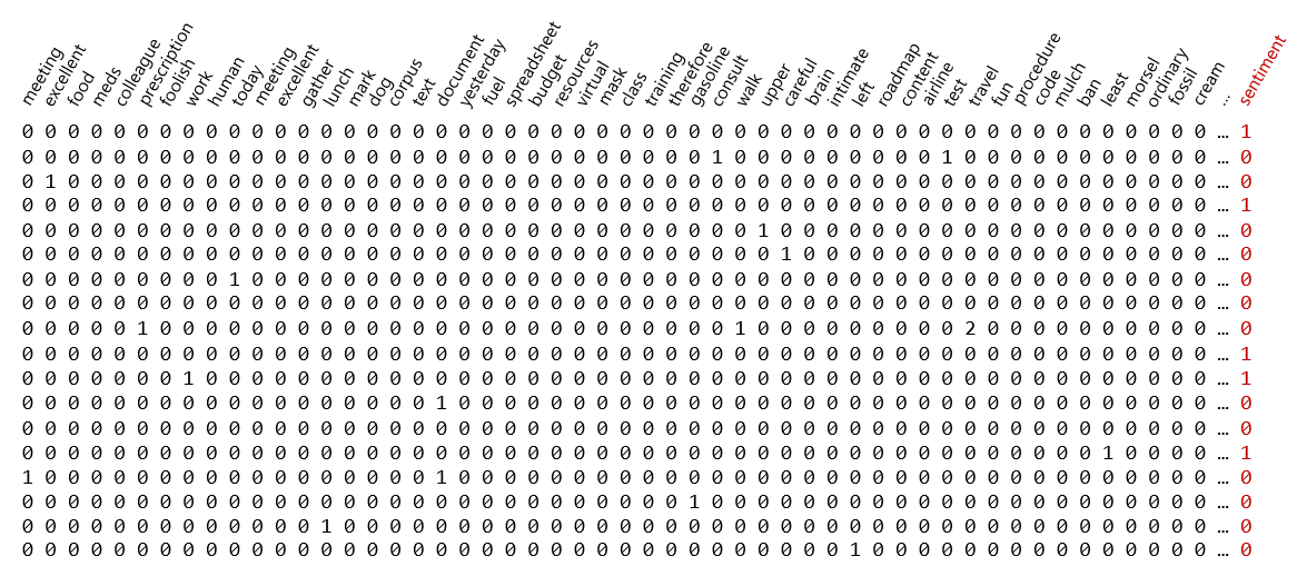
Before it’s vectorized, text is typically cleaned. Examples of cleaning include converting all characters to lowercase (so, for example, “Excellent” doesn’t score differently than “excellent”), removing punctuation symbols and numbers, and removing stop words – common words such as “the” and “and” that are likely to have little bearing on the outcome. Once cleaned, sentences are divided into individual words (“tokenized”) and the words are used to produce a dataset like the one pictured above.
Scikit-learn offers three classes that do the bulk of the work of cleaning and vectorizing text:
- CountVectorizer, which creates a dictionary (“vocabulary”) from a corpus of words provided to it and generates a matrix of word counts like the one above
- HashingVectorizer, which does the same but conserves memory by storing hashes rather than words in the dictionary
- TfidfVectorizer, which creates a dictionary from words provided to it and generates a matrix similar to the one above, but rather than contain integer word counts, the matrix contains Term Frequency-Inverse Document Frequency (TFIDF) values between 0.0 and 1.0 reflecting the relative importance of individual words
All three classes are capable of converting text to lowercase, removing punctuation symbols, removing stop words, splitting sentences into individual words, and more. They also support n-grams, which are combinations of two or more consecutive words (you specify the number n) that should be treated as a single word. The idea is that words such as “credit” and “score” might be more meaningful if they appear next to each other in a sentence than if they appear far apart. Without n-grams, the relative position of words is ignored. (Neural networks have another way of considering word sequences rather than just individual words. I will discuss this in a future post.) The downside to using n-grams is that it increases memory consumption and training time. Used judiciously, it can make text-classification models more accurate.
Here’s an example demonstrating what CountVectorizer does and how it’s used:
import pandas as pd
from sklearn.feature_extraction.text import CountVectorizer

documents = [
    'The quick brown fox',
    'Jumps over $$$ lazy brown dog',
    'Who jumps high into the air',
    'And quickly returns to earth...',
    'Thinking aye aye aye!'
]

# Vectorize the documents
vectorizer = CountVectorizer(stop_words='english')
word_matrix = vectorizer.fit_transform(documents)

# Show the resulting word matrix
feature_names = vectorizer.get_feature_names()
doc_names = [f'Line {idx:d}' for idx, _ in enumerate(word_matrix)]
df = pd.DataFrame(data=word_matrix.toarray(), index=doc_names, columns=feature_names)
df.head()
And here is the output:
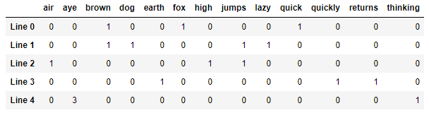
The corpus of text in this case is five sentences in a Python list. CountVectorizer broke the sentences into words, removed stop words and punctuation symbols, and converted the remaining words to lowercase. Those words comprise the columns in the dataset, and the numbers in the rows show how many times a given word appears in each sentence. stop_words=’english’ tells CountVectorizer to remove stop words using a built-in dictionary of more than 300 English-language stop words. If you’d prefer, you can provide your own list of stop words in a Python list. (Or you can leave the stop words in there; it often doesn’t matter.) And if you’re training with text written in another language, you can get lists of multi-language stop words from other Python libraries such as the Natural Language Toolkit (NLTK) and stop-words.
One thing you’ll notice about the output is that “quick” and “quickly” count as separate words, even though they have similar meaning. Data scientists sometimes go a step further when preparing text for machine learning by stemming or lemmatizing words. If the text above were lemmatized, all occurrences of “quickly” would be converted to “quick.” Scikit lacks support for stemming and lemmatization, but you can get it from other libraries such as NLTK.
The example above uses CountVectorizer, which probably has you wondering when (and why) would you use HashingVectorizer or TfidfVectorizer instead? HashingVectorizer is useful when dealing with very large datasets. Rather than store entire words in memory, it stores hashes, and therefore can do more with less memory. The downside to HashingVectorizer is that it doesn’t let you work backwards from vectorized text to the original text. TfidfVectorizer is frequently used in recommendation systems. It assigns weights to words in the training text that reflect their importance, and it uses two factors to determine the weights: how often a word appears in individual documents, and how often it appears in the overall document set. The result is that words that appear more frequently in individual documents but appear in fewer documents are assigned higher weights.
Train a Sentiment-Analysis Model
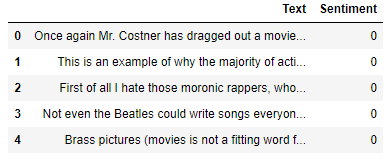
Let’s combine what you learned about Scikit’s LogisticRegression class in the previous post and CountVectorizer in this post to train a sentiment-analysis model. Start by downloading the IMDB movie-review dataset and copying it to the “Data” subdirectory of the directory that hosts your Jupyter notebooks. Then run the following code in a notebook to load the dataset and show the first five rows:
import pandas as pd

df = pd.read_csv('Data/reviews.csv', encoding='ISO-8859-1')
df.head()
Now call info on the DataFrame to see how many samples the dataset contains:
df.info()
There are 50,000 samples. Let’s see how many instances there are of each class (0 for negative and 1 for positive):
df.groupby('Sentiment').describe()
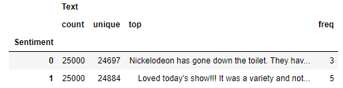
There is an even number of positive and negative samples, but in each case, the number of unique samples in less than the number of samples for that class. That means the dataset has duplicate rows, and duplicate rows could bias a machine-learning model. Use the following statements to delete the duplicate rows and check for balance again:
df = df.drop_duplicates()
df.groupby('Sentiment').describe()
There are no duplicate rows, and there is a roughly even number of positive and negative samples. Let’s use CountVectorizer to prepare and vectorize the text in the “Text” column. Set min_df to 20 to ignore words that appear infrequently in the training text. This will reduce the likelihood of out-of-memory errors and will probably make the model more accurate as well.
from sklearn.feature_extraction.text import CountVectorizer

vectorizer = CountVectorizer(ngram_range=(1, 2), stop_words='english', min_df=20)
x = vectorizer.fit_transform(df['Text'])
y = df['Sentiment']
For an example of what CountVectorizer does, use its transform method to vectorize a line of sample text, and its inverse_transform method to invert the transform and see the result in textual form:
text = vectorizer.transform(['The long l3ines   and; pOOr customer# service really turned me off...123.'])
vectorizer.inverse_transform(text)
Now split the dataset for training and testing. We’ll use a 50/50 split since there are almost 50,000 samples in total:
from sklearn.model_selection import train_test_split

x_train, x_test, y_train, y_test = train_test_split(x, y, test_size=0.5, random_state=0)
The next step is to train a classifier. We’ll use Scikit’s LogisticRegression classifier, which uses logistic regression to fit a model to the data.
from sklearn.linear_model import LogisticRegression

model = LogisticRegression(max_iter=1000, random_state=0)
model.fit(x_train, y_train)
Now validate the trained model with the 50% of the dataset aside for testing and show the results in a confusion matrix:
%matplotlib inline
from sklearn.metrics import plot_confusion_matrix

plot_confusion_matrix(model, x_test, y_test, display_labels=['Negative', 'Positive'], cmap='Blues', xticks_rotation='vertical')
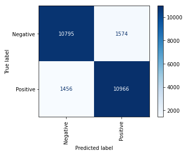
The confusion matrix reveals that the model correctly identified 10,795 negative reviews while misclassifying 1,574 of them. It correctly identified 10,966 positive reviews and got it wrong 1,456 times.
Now comes the fun part: analyzing text for sentiment. Use these statements to produce a sentiment score for the sentence “The long lines and poor customer service really turned me off:”
text = 'The long lines and poor customer service really turned me off'
model.predict_proba(vectorizer.transform([[text]]))[0][1]
Now do the same for “The food was great and the service was excellent:”
text = 'The food was great and the service was excellent'
model.predict_proba(vectorizer.transform([[text]]))[0][1]
Feel free to try sentences of your own and see if you agree with the sentiment scores the model predicts. It’s not perfect, but it’s good enough that if you run hundreds of reviews or comments through it, you should get a pretty reliable indication of the positivity or negativity expressed in the text.
Sometimes using CountVectorizer’s built-in list of English stop words will lower the accuracy of the model because that list is so broad. As an experiment, remove stop_words=’english’ from CountVectorizer and run the code again. Does the accuracy increase or decrease? Feel free to try varying other parameters such as min_df and ngram_range, too. In the real world, data scientists often try many different parameter combinations to determine which one produces the best results.
Get the Code
You can download a Jupyter notebook containing the sentiment-analysis example from the machine-learning repo that I maintain on GitHub. Feel free to check out the other notebooks in the repo while you’re at it. Also be sure to check back from time to time because I am constantly uploading new samples and updating existing ones.
