Most machine-learning models fall into one of two categories. Supervised-learning models make predictions. For example, they predict whether a credit-card transaction is fraudulent or a flight will arrive on time. Unsupervised-learning models don’t make predictions; they provide insights into existing data. The previous post in this series introduced unsupervised learning and used a popular algorithm called k-means clustering to segment customers into groups by age, income level, and other factors for the purpose of identifying customers to target with future marketing campaigns.
Now it’s time to tackle supervised learning. The first thing you should know is that supervised-learning models come in two varieties: regression models and classification models. The purpose of a regression model is to predict a numeric outcome such as the price that a home will sell for or the age of a person in a photo. Classification models, by contrast, predict a class or category from a finite set of classes defined in the training data. Examples include whether a photo contains a picture of a cat or a dog and what number a handwritten digit represents. The former is a binary-classification model because there are just two possible outcomes: the photo contains a cat, or the photo contains a dog. The latter is an example of multiclass classification. Because there are 10 digits (0-9) in the Western Arabic numeral system, there are 10 possible classes that a handwritten digit could represent.
The two types of supervised-learning models are pictured below. On the left, the goal is to input an x and predict what y will be. On the right, the goal is to input an x and a y and predict what class the point corresponds to: a blue triangle or a red ellipse. In both cases, the purpose of applying machine learning to the problem is to build a mathematical model for making predictions. Rather than build that model yourself, you train a machine-learning model with labeled data and allow it to devise a mathematical model for you.
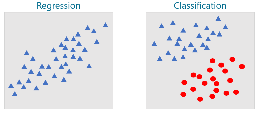
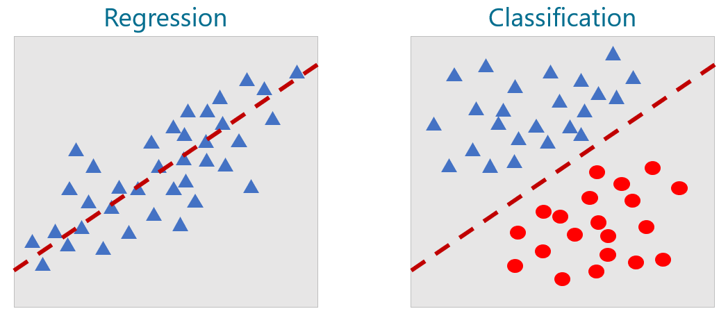
For the datasets above, you could easily build mathematical models without resorting to machine learning. For a regression model, you could draw a line through the data points and use the equation of that line to predict a y given an x. For a classification model, you could draw a line that cleanly separates blue triangles from red ellipses – what data scientists call a separation boundary – and predict which class a new point represents by determining whether the point falls above or below the line. A point just above the line would be classified as a blue triangle, while a point just below it would classify as a red ellipse.
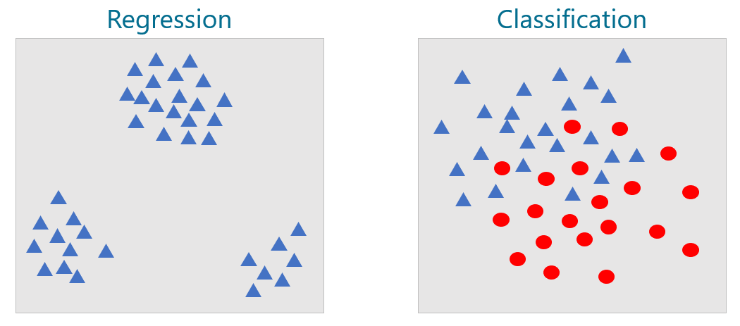
In the real world, datasets are rarely this orderly. They typically look more like the ones below, in which there is no single line you can draw to correlate xs to ys on the left or cleanly separate the classes on the right. The goal, therefore, is to build the best model you can. That means picking the learning algorithm that produces the most accurate model.
There are many supervised-learning algorithms. They go by names such as linear regression, random forests, gradient-boosting machines (GBMs), and support-vector machines (SVMs). Many (but not all) can be used for regression and classification. Even trained data scientists sometimes have to experiment to determine which learning algorithm produces the most accurate predictive model. I will cover many of these algorithms in this series. For now, we will examine perhaps the simplest supervised-learning algorithm of all: k-nearest neighbors.
k-Nearest Neighbors
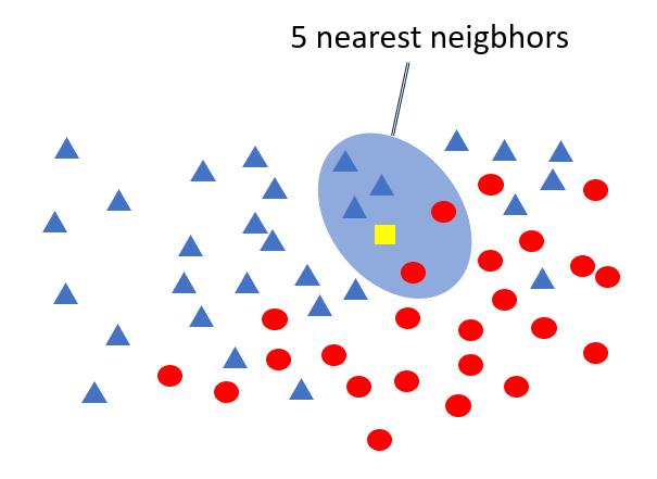
The premise behind k-nearest neighbors is that if you have a set of data points, you can predict a label for a new point by examining the points nearest it. For a regression problem, this means that given an x, you can predict a y by finding the n points with the nearest xs and averaging their ys. For a classification problem, you find the n points closest to the point whose class you want to predict and choose the class with the highest occurrence count. If n=5 and the five nearest neighbors include three blue triangles and two red ellipses, then the answer is a blue triangle as pictured below.
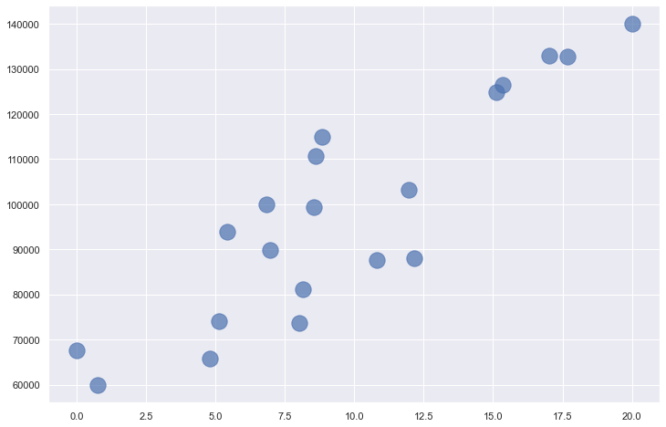
Here’s an example involving regression. Suppose you have 20 data points describing how much programmers earn per year based on years of experience. The diagram below plots years of experience on the x axis and annual income on the y axis. Your goal is to predict what someone with 10 years of experience should earn. In this example, x=10, and you want to predict what y should be.
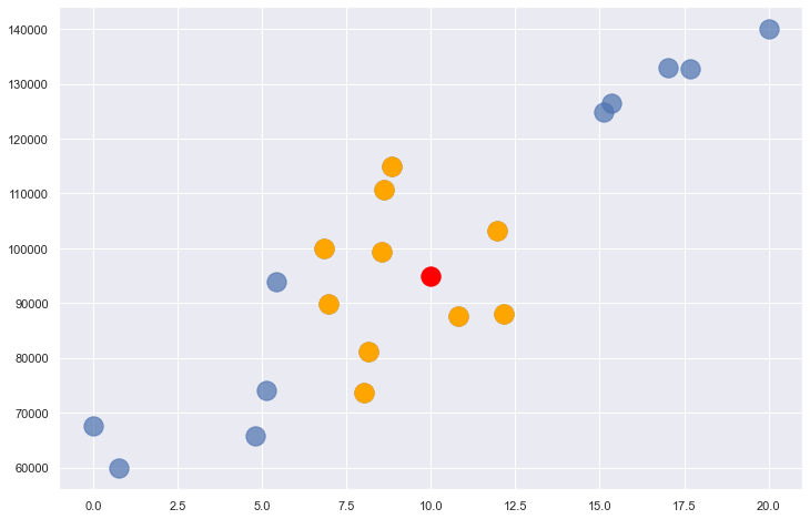
Applying k-nearest neighbors with n=10 identifies the points highlighted in orange as the nearest neighbors – the ten whose x coordinates are closest to x=10. The average of these points’ y coordinates is 94,838. Therefore, k-nearest neighbors with n=10 predicts that a programmer with 10 years of experience will earn $94,838, as indicated by the red dot.
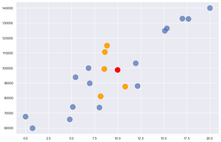
The value of n that you use with k-nearest neighbors influences the outcome. Here’s what the same problem looks like with n=5. The answer is slightly different this time because the average y for the five nearest neighbors is 98,713.
In real life, it’s a little more nuanced because while the dataset has just one label column, it probably has several feature columns – not just x, but x1, x2, x3, and so on. You can compute distances in n-dimensional space easily enough, but there are several ways to measure distances to identify a point’s nearest neighbors, including Euclidean distance, Manhattan distance, and Minkowski distance. You can even use weights so that nearby points contribute more to the outcome more than faraway points. And rather than find the n nearest neighbors, you can select all the neighbors within a given radius, a technique known as radius neighbors. Still, the principle is the same regardless of the number of dimensions in the dataset, the method used to measure distance, and whether you choose n nearest neighbors or all the neighbors within a specified radius: find data points that are similar to the target point and use them to regress or classify the target.
Use k-Nearest Neighbors to Classify Flowers
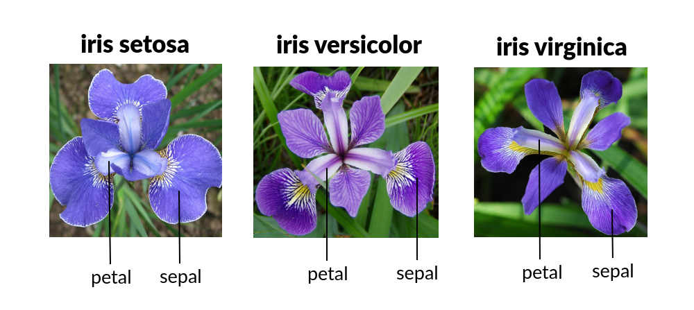
Scikit-learn includes classes named KNeighborsRegressor and KNeighborsClassifier to help you train regression and classification models using the k-nearest neighbors learning algorithm. It also includes classes named RadiusNeighborsRegressor and RadiusNeighborsClassifier that accept a radius rather than a number of neighbors. Let’s look at an example that uses KNeighborsClassifier to classify flowers using the famous iris dataset. That dataset includes 150 samples, each representing one of three species of iris. Each row contains four measurements – sepal length, sepal width, petal length, and petal width, all in centimeters – plus a label: 0 for setosa, 1 for versicolor, and 2 for virginica. Here’s an example of each species along with labels showing the difference between petals and sepals.
To train a machine-learning model to differentiate between specifies of iris based on sepal and petal dimensions, begin by pasting the following code into a Jupyter notebook:
import pandas as pd
import matplotlib.pyplot as plt
import seaborn as sns

sns.set()
%matplotlib inline
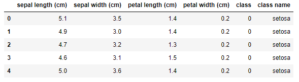
In the next cell, use the following code to load the dataset, wrap a Pandas DataFrame around it, add a column to the DataFrame containing the class name (setosa, versicolor, or virginica), and show the first five rows:
from sklearn.datasets import load_iris

iris = load_iris()
df = pd.DataFrame(iris.data, columns=iris.feature_names)
df['class'] = iris.target
df['class name'] = iris.target_names[iris['target']]
df.head()
The iris dataset is one of several sample datasets included with Scikit. That’s why you can load it by calling Scikit’s load_iris function rather than reading it from an external file. Here’s the output from the code:
Before you train a machine-learning model from the data, you need to split the dataset into two datasets: one for training and one for testing. That’s important, because if you don’t test a model with data it hasn’t seen before – that is, data it wasn’t trained with – you have no idea how accurate it is at making predictions.
Fortunately, Scikit’s train_test_split function makes it easy to split a dataset using a fractional split that you specify. Use the following statements to perform an 80/20 split with 80% of the rows set aside for training and 20% reserved for testing:
from sklearn.model_selection import train_test_split

x_train, x_test, y_train, y_test = train_test_split(iris.data, iris.target, test_size=0.2, random_state=0)
Now, x_train and y_train hold 120 rows of randomly selected measurements and labels, while x_test and y_test hold the remaining 30. 80/20 splits are customary for small datasets like this one, but there’s no rule saying you have to split 80/20. The more data you train with, the more accurate the model is. (That’s not strictly true, but generally speaking, you always want as much training data as you can get.) But the more data you test with, the more confidence you have in measurements of the model’s accuracy. For a small dataset, 80/20 is a reasonable place to start.
The next step is to train a machine-learning model. Thanks to Scikit, that requires just a few lines of code:
from sklearn.neighbors import KNeighborsClassifier

model = KNeighborsClassifier()
model.fit(x_train, y_train)
In Scikit, you create a machine-learning model by instantiating the class encapsulating the learning algorithm you selected – in this case, KNeighborsClassifier. Then you call fit on the model to train it by fitting it to the training data. With just 120 rows of training data, training happens very quickly.
The final step is to use the 30 rows of test data split off from the original dataset to measure the model’s accuracy. In Scikit, that’s accomplished by calling the model’s score method:
model.score(x_test, y_test)
In this example, score returns 0.966667, which means the model got it right about 97% of the time when making predictions with the features in x_test and comparing the predicted labels to the actual labels in y_test.
Of course, the whole purpose of training a predictive model is to make predictions with it. In Scikit, you make a prediction by calling the model’s predict method. Use the following statements to predict the class – 0 for setosa, 1 for versicolor, and 2 for virginica – identifying the species of an iris whose sepal length is 5.6 cm, sepal width is 4.4 cm, petal length is 1.2 cm, and petal width is 0.4 cm:
model.predict([[5.6, 4.4, 1.2, 0.4]])
The predict method can make multiple predictions in a single call. That’s why you pass it a list of lists rather than just a list. It returns a list whose length equals the number of lists you passed in. Since you passed just one list to predict, the return value is a list with one value. In this example, the predicted class is 0, meaning your model predicted that an iris whose sepal length is 5.6 cm, sepal width is 4.4 cm, petal length is 1.2 cm, and petal width is 0.4 cm is mostly likely a setosa iris.
When you create a KNeighborsClassifier without specifying the number of neighbors, it defaults to 5. You can specify the number of neighbors this way:
model = KNeighborsClassifier(n_neighbors=10)
Try fitting (training) and scoring the model again using n_neighbors=10. Does the model score the same? Does predict still predict class 0? Feel free to experiment with other n_neighbors values to get a feel for their effect on the outcome.
The process that you used here – load the data, split the data, create a classifier or regressor, call fit to fit it to the training data, call score to assess the model’s accuracy using test data, and finally, call predict to make predictions – is one that you will use over and over with Scikit. In the real world, data frequently requires cleaning before it’s used for training and testing. You’ll see plenty of examples of that later, but in this example, the data was complete and well-structured right out of the box and therefore required no cleaning.
KNeighborsClassifier Internals
k-nearest neighbors is sometimes referred to as a lazy learning algorithm because most of the work is done when you call predict rather than when you call fit. In fact, training technically doesn’t have to do anything except make a copy of the training data for when predict is called. So what happens inside KNeighborsClassifier when you call fit?
In most cases, fit constructs a binary tree in memory that makes predict faster by preventing it from having to perform a brute-force search. The tree is either a k-d tree or a ball tree, and if you prefer one over the other, you can specify the tree type using KNeighborsClassifier’s algorithm parameter. The default is “auto,” which lets KNeighborsClassifier choose the tree type. If KNeighborsClassifier determines that neither a k-d tree nor a ball tree will help, then it skips the tree building and resorts to brute-force searches when predict is called. This typically happens when the training data is sparse – that is, it is mostly zeroes with a few non-zero values sprinkled in.
One of the wonderful things about Scikit-learn is that it is open-source. If you care to know more about how a particular class or method works, you can go straight to the source code. The code is hosted on GitHub. You’ll find the source code for KNeighborsClassifier and RadiusNeighborsClassifier here.
Get the Code
You can download a Jupyter notebook containing the iris-dataset example from the machine-learning repo that I maintain on GitHub. Feel free to check out the other notebooks in the repo while you’re at it. I’ll be using some of them in future posts. Be sure to check back from time to time because I am constantly uploading new samples and updating existing ones.
