Supervised-learning models come in two varieties: regression models and classification models. Regression models predict numeric outcomes, such as the price of a car. Classification models predict classes, such as the breed of a dog in a photo.
When you build a machine-learning model, the first and most important decision you make is what learning algorithm to use to learn from the training data. In the previous post, I presented a simple 3-class classification model that used the k-nearest neighbors learning algorithm to identify a species of iris given the flower’s sepal and petal measurements. In this post, we learn about common regression algorithms, many of which can be used for classification, too. We also learn about one of the most egregious problems of all in machine learning: overfitting.
Linear Regression
Next to k-nearest neighbors, linear regression is perhaps the simplest learning algorithm of all. It works best with data that is relatively linear – that is, data points that fall roughly along a line. If you think back to high-school math class, you’ll recall that the equation for a line is:
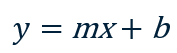
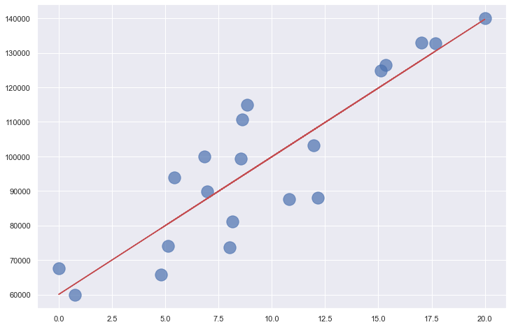
Where m is the slope of the line, and b is where the line intersects the y axis. The income-versus-years-of-experience dataset featured in the previous post lends itself well to linear regression. The illustration below shows a regression line fit to the data points. Predicting the income for a programmer with 10 years of experience is as simple as finding the point on the line where x=10. The equation of the line is y = 3,984x + 60,040. Plugging 10 into that equation for x, the predicted income is $99,880.
The goal when training a linear-regression model is finding values for m and b that produce the most accurate predictions. This is typically done using an iterative process that starts with assumed values for m and b and repeats until it converges on suitable values. The most common technique for fitting a line to a set of points is ordinary least-squares regression, or OLS for short. OLS works by squaring the distance in the y direction between each point and the regression line (among other things, squaring each distance prevents negative distances from offsetting positive distances), summing the squares, and dividing by the number of points to compute the mean squared error, or MSE. Then it adjusts m and b to reduce MSE the next time around and repeats until MSE is sufficiently small. I won’t go into the details of how it determines which direction to adjust m and b (it’s not hard, but it involves a smidgeon of calculus – specifically, first derivatives), but OLS can often fit a line to a set of points with a dozen or fewer iterations.
Scikit has a number of classes to help you build linear-regression models, including the LinearRegression class, which embodies OLS. Training a linear-regression model can be simple as this:
model = LinearRegression()
model.fit(x, y)
Scikit has many other linear-regression classes with names such as Ridge and Lasso. I won’t cover them in this post, but they’re sometimes useful when, for example, you have datasets with outliers and you want to mitigate the effect of those outliers, an act that data scientists refer to as regularization. It also includes a class named PolynomialFeatures for doing polynomial regression, which fits a polynomial curve rather than a straight line to training data.
Linear regression isn’t limited to two dimensions (xs and ys); it works with any number of dimensions. If the dataset is 2-dimensional, it’s simple enough to plot the data to determine how linear it is. You can plot 3-dimensional data, too, but good luck figuring out how to plot datasets with 4 or 5 dimensions, much less datasets with hundreds or thousands of dimensions.
How do you determine whether a high-dimensional dataset might lend itself to linear regression? One way to do it is to reduce n dimensions to 2 or 3 using techniques such as principal component analysis (PCA) and t-distributed stochastic neighbor embedding (t-SNE) so you can plot them. These techniques are beyond the scope of this article but will be covered in a later post. Both reduce the dimensionality of a dataset without a commensurate loss of information. With PCA, for example, it isn’t uncommon to reduce the number of dimensions by 90% while retaining 90% of the information in the original dataset. If it sounds like magic, it’s not. It’s math.
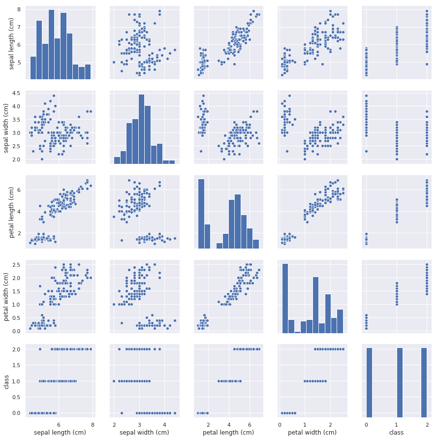
A simpler technique for visualizing high-dimensional datasets if the number of dimensions n is small is pair plots, which plot pairs of dimensions in conventional 2-dimensional charts. Here’s a pair plot showing sepal length vs. petal length, sepal width vs. petal width, and other parameter pairs for the iris dataset featured in my previous post:
An easy way to create pair plots is to use Seaborn’s pairplot function. The pair plot above was generated with one simple line of code:
sns.pairplot(df)
The pair plot not only helps us visualize relationships in the dataset, but in this example, the histogram in the lower-right corner reveals that the dataset is balanced, too. There is an equal number of samples of all three classes, and for reasons you will learn later on when we delve more deeply into classification models, you always prefer to train classification models with balanced datasets.
Linear regression is a parametric learning algorithm, which means that its purpose is to examine a dataset and find the optimum values for parameters in an equation – for example, m and b. k-nearest neighbors, by contrast, is a non-parametric learning algorithm because it doesn’t fit data to an equation. Why does it matter whether a learning algorithm is parametric or non-parametric? Because datasets used to train parametric models frequently need to be normalized. At its simplest, normalizing data means making sure all the values in all the columns have consistent ranges. I’ll cover normalization in a separate post later on, but for now, realize that training parametric models with unnormalized data – for example, a dataset that contains values from 0 to 1 in one column and 0 to 1,000,000 in another – sometimes makes those models less accurate or prevents them from converging on a solution altogether. This is particularly true with support-vector machines and neural networks, but it applies to other types of parametric models as well.
Decision Trees
Even if you’ve never taken a computer-science course, you probably know what a binary tree or is. In machine learning, a decision tree is a binary tree that lets you answer a question by answering a series of yes/no questions.
The graphic below shows a decision tree built by Scikit from the income-versus-experience dataset in my previous post. The tree is simple because the dataset contains just one feature column (years of experience) and I purposely limited the tree’s depth to 3, but the technique extends to trees of infinite size and complexity. In this example, predicting a salary for a programmer with 10 years of experience requires just three yes/no decisions as indicated by the red arrows. The answer is about $100K, which is pretty close to what k-nearest neighbors and linear regression predicted when applied to the same dataset.
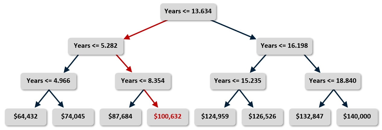
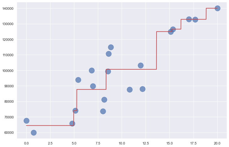
Decision trees can be used for regression and classification. For a regressor, the leaf nodes (the nodes that lack children) represent regression values. For a classifier, they represent classes. The output from a decision-tree regressor isn’t continuous. The output will always be one of the values assigned to a leaf node, and there is a finite number of leaf nodes. The output from a linear-regression model, by contrast, is continuous. It can assume any value along the line fit to the training data. In the example above, you get the same answer if you ask the tree to predict a salary for someone with 10 years of experience and someone with 13.6 years of experience. Bump years of experience up to 13.7, however, and the predicted salary jumps to $125K (see below). If you allow the tree to grow deeper, the answers become more refined. But allowing it to grow too deep can lead to big problems, as you’ll learn momentarily.
Once a decision-tree model is trained – that is, once the tree is built – predictions are fast. But how do you decide what decisions to make at each node? For example, why is the number of years represented by the root node in the illustration above 13.634? Why not 10.000 or 8.742 or some other number? For that matter, if the dataset has multiple feature columns, how do you decide which column to break on at each decision node?
The fundamental decision that the algorithm makes when it adds a node to the tree is 1) Which column will this node split, and 2) what is the value that the split is based upon? The math works differently for regressors and classifiers, but in each case, a value is computed for each feature column that quantifies the variance in the output (the values in the label column) attributable to that column. The split is typically done on the feature column exhibiting the lowest variance, and the split value is determined by imputing a value in the feature column that corresponds to the mean of the values in the label column. Each split reduces the variance in the remaining output and moves us one step closer to the answer. This process starts at the root node and works its way recursively downward until the tree is fully leafed out or external constraints (such as a limit on maximum depth) prevent further growth.
Scikit’s DecisionTreeRegressor and DecisionTreeClassifier classes make building decision trees easy. Each lets you choose from a handful of algorithms for computing variance. And each includes attributes such as max_depth, min_samples_split, and min_samples_leaf that let you constrain a decision tree’s growth. If you accept the default values, building a decision tree can be as simple as this:
model = DecisionTreeRegressor()
model.fit(x, y)
Decision trees are non-parametric. Training a decision-tree model involves building a binary tree, not fitting an equation to a dataset. This means that data used to build a decision tree doesn’t have to be normalized. Once more, you’ll learn all about normalization in a future post.
Decision trees have a big upside: they work as well with non-linear data as they do with linear data. In fact, they largely don’t care how the data is shaped. But there’s a downside, too. It’s a big one, and it’s one of the reasons stand-alone decision trees are rarely used in machine learning. That reason is overfitting.
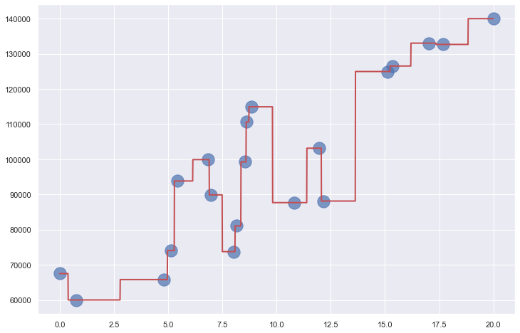
Decision trees are highly prone to overfitting. If allowed to grow large enough, a decision tree can essentially memorize the training data. It might appear to be accurate, but if it’s fit too tightly to the training data, it might not generalize well. That means it won’t be as accurate when it’s asked to make predictions with data it has never seen before. The plot below shows a decision tree fit to the income-versus-experience dataset with no constraints on depth. The jagged path followed by the red line as it passes through all the points is a clear sign of overfitting. Overfitting is the bane of data scientists, and something that one must always guard against. The only thing worse than a model that’s inaccurate is one that appears to be accurate, but in reality is not.
One way to prevent overfitting when you use decision trees is to constrain their growth so they can’t memorize the training data. Another way is to use groups of decision trees called random forests.
Random Forests
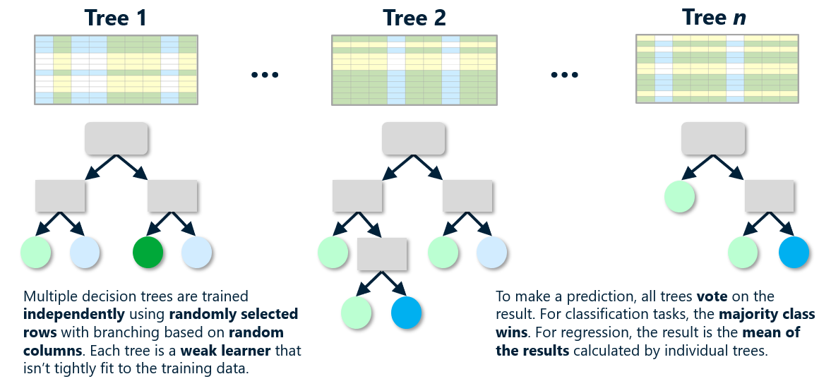
A random forest is a collection of decision trees (often hundreds of them), each trained differently on the same data. Typically, each tree is trained on randomly selected rows in the dataset, and branching is based on columns that are randomly selected at every split. The model can’t fit too tightly to the training data because every tree sees the data differently. The trees are built independently, and when the model makes a prediction, it runs the input through all the decision trees and averages the result. Because the trees are constructed independently, training can be parallelized on hardware that supports it.
It’s a simple concept, and one that works well in the real world. Random forests can be used for both regression and classification, and Scikit provides helpful classes such as RandomForestRegressor and RandomForestClassifier to help out. These classes feature a number of tunable parameters, including n_estimators, which specifies the number of trees in the random forest (default=100); max_depth, which limits the depth of each tree; and max_samples, which specifies the fraction of the rows in the training data used to build individual trees. The chart below shows how RandomForestRegressor fits to the income-versus-experience dataset with max_depth=3 and max_samples=0.5, meaning no tree sees more than 50% of the rows in the dataset.
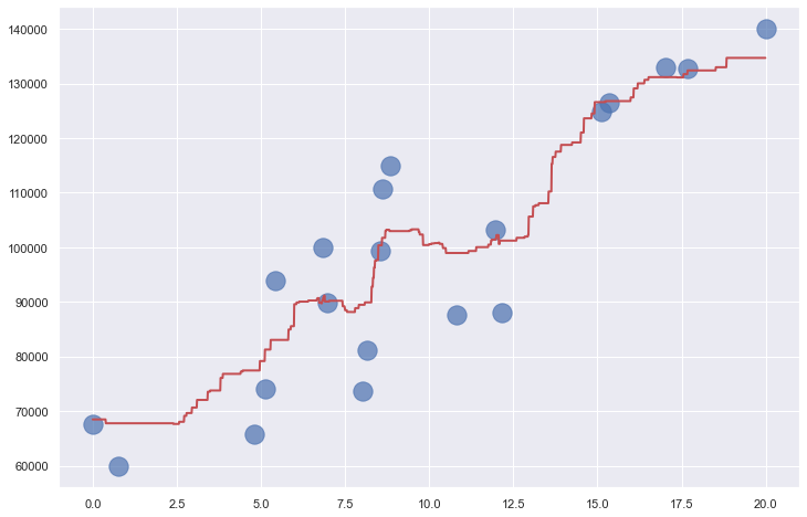
Because decision trees are non-parametric, random forests are non-parametric also. Even though the diagram above shows how a random forest fits a linear dataset, keep in mind that random forests are perfectly capable of fitting much less structured datasets.
Gradient-Boosting Machines
Random forests are proof of the supposition that you can take many weak learners – models that by themselves are not strong predictors – and combine them to form accurate models. No individual tree in a random forest can predict an outcome with a great deal of accuracy. But put all the trees together and average the results and they often outperform other models. Data scientists refer to this as ensemble modeling or ensemble learning.
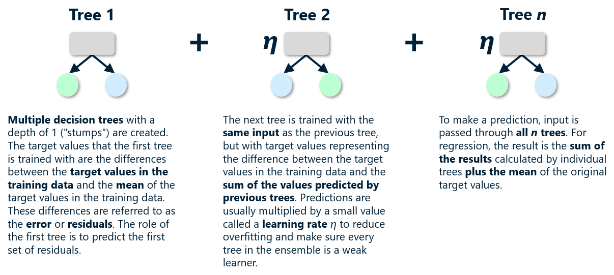
Another way to exploit ensemble modeling is gradient boosting. Models that use it are called gradient-boosting machines, or GBMs. Most GBMs use decision trees and are sometimes referred to as gradient-boosted decision trees (GBDTs). Like random forests, GBDTs comprise collections of decision trees. But rather than build independent decision trees from random subsets of the data, GBDTs build dependent decision trees, one after another, training each using output from the last. The first decision tree models the dataset. The second decision tree models the error in the output from the first, the third models the error in the output from the second, and so on. To make a prediction, a GBDT runs the input through each decision tree and sums all the outputs to arrive at a result. With each addition, the result becomes slightly more accurate, giving rise to the term additive modeling. It’s like driving a golf ball down the fairway and hitting successively shorter shots until you finally reach the hole.
Each decision tree in a GBDT model is a weak learner. In fact, GBDTs typically use decision-tree stumps, which are decision trees with depth 1 (a root node and two child nodes). During training, you start by taking the mean of all the target values in the training data to create a baseline set of predictions. Then you subtract the mean from the target values to generate a new set of target values or residuals for the first tree to predict. After training the first tree, you run the input through it to generate a set of predictions. Then you add the predictions to the previous set of predictions, generate a new set of residuals by subtracting the sum from the original (actual) target values, and train a second tree to predict those residuals. Repeating this process for n trees, where n is typically 100 or more, produces an ensemble model. To help ensure that each decision tree is a weak learner, GBDT models multiply the output from each decision tree by a learning rate to reduce their influence on the outcome. The learning rate is usually a small number such as 0.1 and is a parameter than you can specify when using classes that implement GBMs.
Scikit includes classes named GradientBoostingRegressor and GradientBoostingClassifier to help you build GBDTs. But if you really want to understand how GBDTs work, you can build one yourself with Scikit’s DecisionTreeRegressor class. The following code implements a GBDT with 100 decision-tree stumps and predicts the annual income of a programmer with 10 years of experience:
learning_rate = 0.1 # Learning rate
n_trees = 100 # Number of decision trees
trees = [] # Trees that comprise the model

# Compute the mean of all the target values
y_pred = np.array([y.mean()] * len(y))
baseline = y_pred

# Create n_trees and train each with the error in the output from the previous tree
for i in range(n_trees):
    error = y - y_pred
    tree = DecisionTreeRegressor(max_depth=1, random_state=0)
    tree.fit(x, error)
    predictions = tree.predict(x)
    y_pred = y_pred + (learning_rate * predictions)
    trees.append(tree)

# Predict a y for x=10
y_pred = np.array([baseline[0]] * len(x))

for tree in trees:
    y_pred = y_pred + (learning_rate * tree.predict([[10.0]]))

print(y_pred[0])
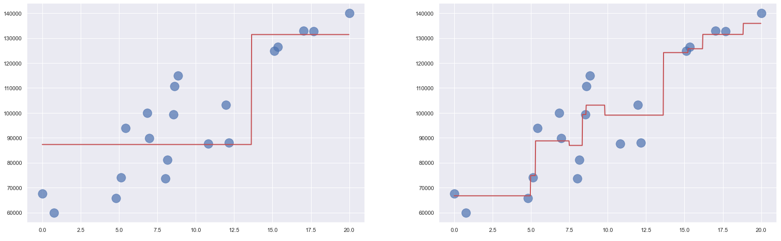
The diagram on the left below shows the output from a single decision-tree stump applied to our income-versus-experience dataset. That model is such a weak learner that it can only predict two different income levels. The diagram on the right shows the output from the model above. The additive effect of the weak learners produces a strong learner that predicts a programmer with 10 years of experience should earn $99,082 per year, which is consistent with the predictions made by other models we have examined.
GBDTs can be used for regression and classification, and they are non-parametric. Aside from neural networks and support-vector machines, GBDTs are frequently the ones that data scientists find most capable of modeling complex datasets.
Linear-regression models do not overfit. Random forests rarely overfit, especially if individual trees are trained on subsets of the data. Decision trees are prone to overfitting, and GBDTs are somewhat prone, too. One way to mitigate that when using GradientBoostingRegressor and GradientBoostingClassifier is to use the subsample parameter to prevent individual trees from seeing the entire dataset, analogous to what max_samples does for random forests. Another way is to use the learning_rate parameter to lower the learning rate, which defaults to 0.1.
Support-Vector Machines
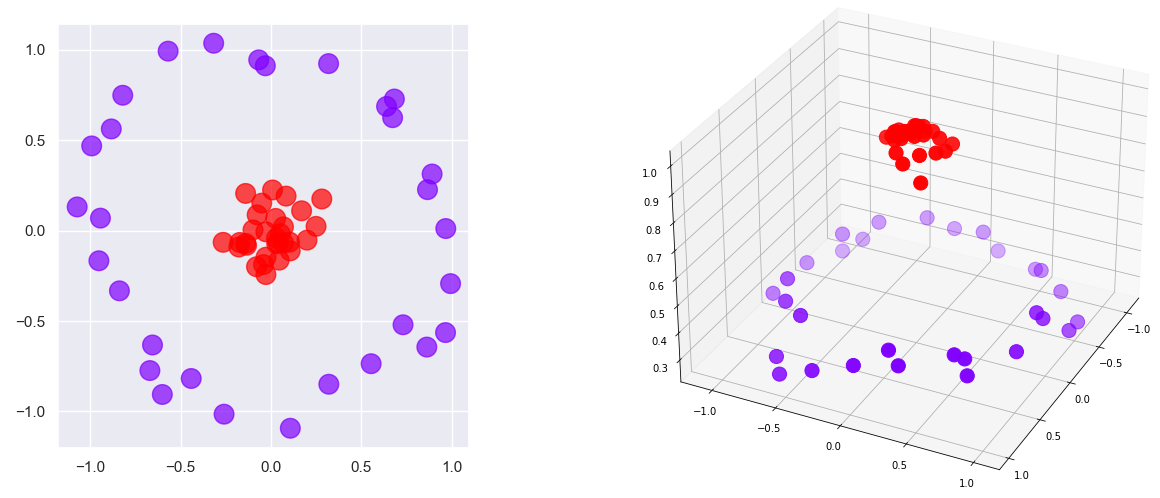
I will save a full treatment of support-vector machines (SVMs) for a future post, but along with GBMs, they represent the cutting edge of statistical machine learning. They can often fit models to highly non-linear datasets that other learning algorithms cannot. They’re so important that they merit separate treatment from all other algorithms. They work by employing a mathematical device called kernel tricks to add dimensions to data. The idea is that data that isn’t separable in m dimensions might be separable in n dimensions. Here’s a quick example.
The classes in the 2-dimensional dataset on the left side of the diagram below can’t be separated with a line. But if you add a third dimension so that points closer to the center have higher z values and points farther from the center have lower z values as shown on the right, you can slide a plane between the red points and the purple points and achieve 100% separation of the classes. That is the principle by which SVMs work. It is mathematically complex when generalized to work with arbitrary datasets, but it is an extremely powerful technique that is vastly simplified by Scikit.
SVMs are primarily used for classification, but they can be used for regression as well. Scikit includes classes for doing both, including SVC for classification problems and SVR for regression problems. You will learn all about these classes later. For now, drop the term “support-vector machine” at the next machine-learning party you attend and you will instantly become the life of the party.
In my next post, we will put some of these learning algorithms to work building a very cool regression model and training it with a dataset drawn from real-world data.
