One of the common uses for machine learning is performing binary classification, which looks at an input and predicts which of two possible classes it belongs to. Practical uses include sentiment analysis, spam detection, and credit-card fraud detection. Such models are trained with datasets labeled with 1s and 0s representing the two classes, employ popular learning algorithms such as logistic regression and Naïve Bayes, and are frequently built with libraries such as Scikit-learn.
Deep learning can be used for binary classification, too. In fact, building a neural network that acts as a binary classifier is little different than building one that acts as a regressor. In this post, you’ll learn how to use Keras to build binary classifiers. My next post will describe how to create deep-learning models that perform multiclass classification.
Building a Binary Classifier
In the previous post in this series, you learned how to build a neural network to solve a regression problem. That network had an input layer that accepted three values – distance to travel, hour of day, and day of week – and output a predicted taxi fare. Here’s how that network was defined using Keras’s sequential API:
model = Sequential()
model.add(Dense(512, activation='relu', input_dim=3))
model.add(Dense(512, activation='relu'))
model.add(Dense(1))
model.compile(optimizer='adam', loss='mae', metrics=['mae'])
Building a neural network that performs binary classification involves making two simple changes:
- Add an activation function – specifically, the sigmoid activation function – to the output layer. Sigmoid reduces the output to a value from 0.0 to 1.0 representing a probability. For a reminder of what a sigmoid function does, see my post on binary classification.
- Change the loss function to binary_crossentropy, which is purpose-built for binary classifiers. Accordingly, change metrics to ‘accuracy’ so accuracies computed by the loss function are captured in the history object returned by fit.
Here’s an equivalent network designed to perform binary classification rather than regression:
model = Sequential()
model.add(Dense(512, activation='relu', input_dim=3))
model.add(Dense(512, activation='relu'))
model.add(Dense(1, activation='sigmoid'))
model.compile(optimizer='adam', loss='binary_crossentropy', metrics=['accuracy'])
That’s it. That’s all it takes to create a neural network that serves as a binary classifier. You still call fit to train the network, and you use the returned history object to plot the training and validation accuracy to determine whether you trained for a sufficient number of epochs and see how well the network fit to the data.
To sum up, you build a neural network that performs binary classification by including a single neuron with sigmoid activation in the output layer and specifying binary_crossentropy as the loss function. The output from the network is a probability from 0.0 to 1.0 that the input belongs to the positive class. Doesn’t get much simpler than that!
What is binary cross-entropy, and what does it do to help a binary classifier converge on a solution? During training, the cross-entropy loss function exponentially increases the penalty for wrong outputs to drive the weights and biases more aggressively in the right direction.
Let’s say a sample belongs to the positive class (its label is 1), and the network predicts that the probability it’s a 1 is 0.9. The cross-entropy loss, also known as log loss, is –log(0.9), which is 0.04. But if the network outputs a probability of 0.1 for the same sample, the error is –log(0.1), which equals 1. What’s significant is that if the predicted probability is really wrong, the penalty is much higher. If the sample is a 1 and the network says the probability it’s a 1 is a mere 0.0001, the cross-entropy loss is –log(0.0001), or 4. Cross-entropy loss basically pats the optimizer on the back when it’s close to the right answer and slaps it on the hand when it’s not. The worse the prediction, the harder the slap.
Making Predictions
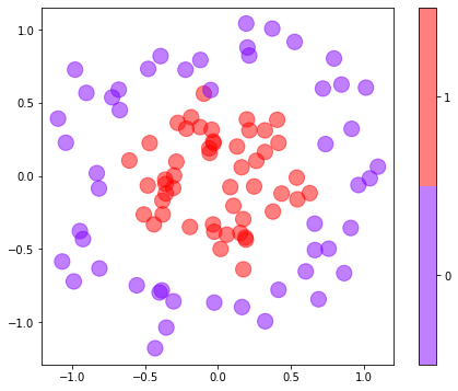
One of the benefits of a neural network is that it can easily fit non-linear datasets. You don’t have to worry about trying different learning algorithms as you do with conventional machine-learning models; the network is the learning algorithm. As an example, consider the dataset below, in which each data point consists of an x–y coordinate pair and belongs to one of two classes:
The following code trains a neural network to predict a class based on a point’s x and y coordinates:
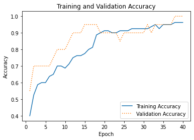
model = Sequential()
model.add(Dense(128, activation='relu', input_dim=2))
model.add(Dense(1, activation='sigmoid'))
model.compile(optimizer='adam', loss='binary_crossentropy', metrics=['accuracy'])
hist = model.fit(x, y, epochs=40, batch_size=10, validation_split=0.2)
This network contains just one hidden layer with 128 neurons. And yet a plot of the training and validation accuracy reveals that it is remarkably successful in separating the classes:
Once a binary classifier is trained, you make predictions by calling its predict method. Thanks to the sigmoid activation function, predict returns a number from 0.0 to 1.0 representing the probability that the input belongs to the positive class. In this example, purple data points represent the negative class (0), while red data points represent the positive class (1). Here, the network is asked to predict the probability that a data point at (-0.5, 0.0) belongs to the red class:
model.predict(np.array([[-0.5, 0.0]]))
The answer is 0.57, which indicates that (-0.5, 0.0) is more likely to be red than purple. If you simply want to know which class the point belongs to, do it this way:
(model.predict(np.array([[-0.5, 0.0]])) > 0.5).astype('int32')
The answer is 1, which corresponds to red. Older versions of Keras included a predict_classes method that did the same without the astype cast, but that method was recently deprecated and removed.
Train a Neural Network to Detect Credit-Card Fraud
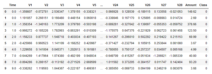
Let’s build a neural network that detects credit-card fraud. Start by downloading the zip file containing the dataset and extracting creditcard.csv from the zip file. (The CSV file is larger than the 100 MB maximum that GitHub allows, so I zipped it up before checking it in.) The dataset is the same one presented in my post on PCA-based anomaly detection. It contains information about 284,808 actual credit-card transactions, including the amount of each transaction and a label: 0 for legitimate transactions, and 1 for fraudulent transactions. It also contains 28 columns named “V1” through “V28” whose meaning has been obfuscated with principal component analysis. The dataset is highly imbalanced, containing just 492 examples of fraudulent transactions.
Drop creditcard.csv into the directory where your Jupyter notebooks are hosted. Then use the following code to load the dataset:
import pandas as pd

df = pd.read_csv('creditcard.csv')
df.head(10)
Use the following statements to drop the “Time” column, divide the dataset into features x and labels y, and split the dataset into two datasets: one for training and one for testing. Rather than allow Keras to do the split for us, we’ll do it ourselves so we can later run the test data through the network and use a confusion matrix to analyze the results:
from sklearn.model_selection import train_test_split

x = df.drop(['Time', 'Class'], axis=1)
y = df['Class']

x_train, x_test, y_train, y_test = train_test_split(x, y, test_size=0.2, stratify=y, random_state=0)
Create a neural network for binary classification:
from keras.models import Sequential
from keras.layers import Dense

model = Sequential()
model.add(Dense(128, activation='relu', input_dim=29))
model.add(Dense(1, activation='sigmoid'))
model.compile(loss='binary_crossentropy', optimizer='adam', metrics=['accuracy'])
model.summary()
The next step is to train the model. Notice the validation_data parameter passed to fit, which uses the test data split off from the larger dataset to assess the model’s accuracy as training takes place:
hist = model.fit(x_train, y_train, validation_data=(x_test, y_test), epochs=10, batch_size=100)
Now plot the training and validation accuracy using the per-epoch values in the history object:
import matplotlib.pyplot as plt
%matplotlib inline
import seaborn as sns
sns.set()

acc = hist.history['accuracy']
val = hist.history['val_accuracy']
epochs = range(1, len(acc) + 1)

plt.plot(epochs, acc, '-', label='Training accuracy')
plt.plot(epochs, val, ':', label='Validation accuracy')
plt.title('Training and Validation Accuracy')
plt.xlabel('Epoch')
plt.ylabel('Accuracy')
plt.legend(loc='lower right')
plt.plot()
The result looked like this for me. Remember that your results will be different thanks to the randomness inherent to training neural networks:
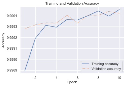
On the surface, the validation accuracy (around 0.9994) appears to be very high. But remember that we’re dealing with an imbalanced dataset. Fraudulent transactions represent less than 0.2% of all the samples, which means that the model could simply guess that every transaction is legitimate and get it right about 99.8% of the time. Use a confusion matrix to visualize how the model performs during testing with data it wasn’t trained with:
from sklearn.metrics import confusion_matrix

y_predicted = model.predict(x_test) > 0.5
mat = confusion_matrix(y_test, y_predicted)
labels = ['Legitimate', 'Fraudulent']

sns.heatmap(mat, square=True, annot=True, fmt='d', cbar=False, cmap='Blues',
            xticklabels=labels, yticklabels=labels)

plt.xlabel('Predicted label')
plt.ylabel('Actual label')
You can’t use Scikit’s plot_confusion_matrix function here because it only works with Scikit classifiers, but you can use Scikit’s confusion_matrix function to generate a raw confusion matrix and plot it yourself. Here’s how it turned out for me:
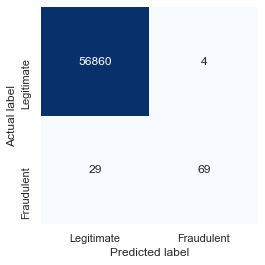
Your results will probably vary. Indeed, if you train the model multiple times, you’ll get different results each time. In this run, the model correctly identified 56,860 transactions as legitimate while misclassifying legitimate transactions just 4 times. This means legitimate transactions are classified correctly more than 99.99% of the time. Meanwhile, the model caught 70% of the fraudulent transactions. That’s acceptable, because credit-card companies would rather allow 100 fraudulent transactions to go through than decline one legitimate transaction. The latter, after all, creates unhappy customers.
Get the Code
You can download a Jupyter notebook containing the fraud-detection example from the deep-learning repo that I maintain on GitHub. Feel free to check out the other notebooks in the repo while you’re at it. Also be sure to check back from time to time because I am constantly uploading new samples and updating existing ones.
