Anomaly detection is a branch of machine learning that seeks to identify anomalies in datasets or data streams. Airbus uses it to predict failures in jet engines and detect anomalies in telemetry data beamed down from the International Space Station. Credit-card companies use it to detect credit-card fraud. The goal of anomaly detection is to identify outliers in data – samples that aren’t “normal” when compared to others. In the case of credit-card fraud, the assumption is that if transactions are subjected to an anomaly-detection algorithm, fraudulent transactions will show up as anomalous, while legitimate transactions will not.
There are many ways to perform anomaly detection. They go by names such as isolation forests, one-class SVMs, and local outlier factor (LOF). Most rely on unsupervised-learning methods and therefore do not require labeled data. They simply look at a collection of samples and determine which ones are anomalous. Unsupervised anomaly detection is particularly interesting because it doesn’t require a priori knowledge of what constitutes an anomaly, nor does it require an unlabeled dataset to be meticulously labeled.
One of the most popular forms of anomaly detection relies on principal component analysis (PCA). My previous post introduced PCA and demonstrated two practical uses for it: removing noise from data and reducing data to 2 or 3 dimensions so it can be visualized and explored. This time, we’ll put PCA to work in an entirely different context.
You already know that PCA can be used to reduce data from m dimensions to n, and that a PCA transform can be inverted to restore the original m dimensions. You also know that inverting the transform doesn’t recover the data lost when the transform was applied. The gist of PCA-based anomaly detection is that an anomalous sample should exhibit more loss or reconstruction error than a normal one. In other words, the loss incurred when an anomalous sample is PCAed and un-PCAed should be higher than the loss incurred when the same operation is applied to a normal sample. Let’s see if this assumption holds up in the real world.
Using PCA to Detect Credit-Card Fraud
One of the life events that got me interested in machine learning happened 10 years ago when I received a call from American Express. Every few years, someone steals my credit-card number and tries to use it to make a purchase. Invariably, American Express calls me, confirms that the transaction was fraudulent, and cancels that card and sends me a new one. Most of the time, it’s easy to detect that something’s amiss, as in the time someone attempted to use my card to buy a plane ticket in a country thousands of miles away.
But on this day, someone tried to buy a necklace at a jewelry store just two miles from my house. I confirmed that it wasn’t me, but I was curious how American Express knew. It turned out that they run every transaction through a sophisticated machine-learning model that is adept at detecting credit-card fraud. But I had to know: how does a model like this work? And how do you build one?
Machine learning isn’t hard when you have a properly engineered dataset to work with. Not surprisingly, companies that use ML to spot credit-card fraud guard their models and the data with which they train them. But at least one such dataset has been published for public consumption. The data in it was anonymized with PCA and then normalized. Most of the columns have uninformative names such as V1 and V2 and contain similarly opaque numbers. Three columns – Time, Amount, and Class – have real names and unaltered values revealing when the transaction took place, the amount of the transaction, and whether the transaction was legitimate (0) or fraudulent (1).
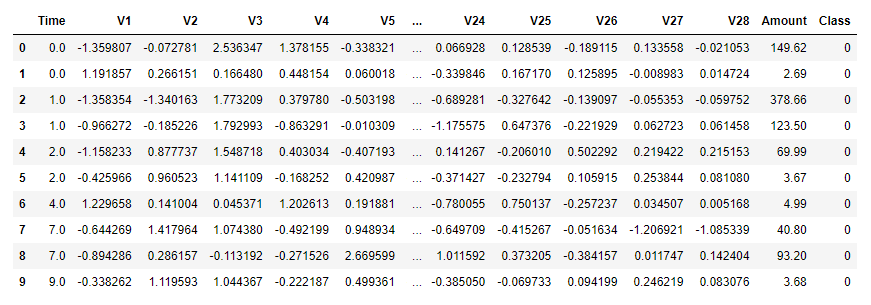
The data comes from real transactions made by European credit-card holders in September 2013. Each row represents one transaction. Of the 284,807 transactions in the dataset, only 492 are fraudulent. The dataset is highly imbalanced, so you would expect a machine-learning model trained on it to be much better at classifying legitimate transactions than fraudulent transactions. That’s not necessarily a problem, because credit-card companies don’t want to anger their customers. They would rather let 100 fraudulent transactions slip through undetected than inconvenience a card-holder by declining a legitimate transaction.
As an aside, this dataset exemplifies another great use case for principal component analysis. Because most of the columns have been PCAed, their content is ostensibly meaningless. But you can still build a machine-learning model from them because all of the information in the original dataset is still there. You don’t know what the original columns held (they probably contained sensitive information such as credit scores and annual incomes), so you can’t use a model trained on them to make predictions. You can, however, experiment with different learning algorithms to determine which one produces the most accurate model.
Here’s a simple code snippet that demonstrates how PCA is used to hide information:
data = [[100, 200, 300], [200, 750, 100], [600, 450, 200]]
pca = PCA(n_components=3)
pca_data = pca.fit_transform(data)
The original dataset contains three rows and three columns. PCA is used to “reduce” it to three columns. Here’s how it looks before and after:
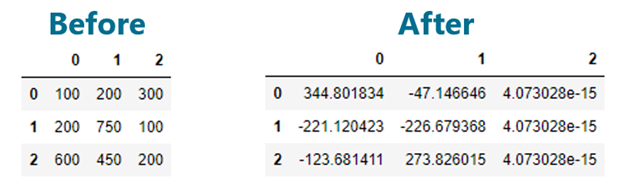
The dataset is virtually unrecognizable after the PCA transform. Without the transform, it’s impossible to work backward and reconstruct the original dataset. Yet the sum of the explained_variance_ratio_ values is 1.0, which means that no information was lost. The PCAed dataset is just as useful for machine learning as the original – once more, with the caveat that you can’t use it to make predictions because you don’t know what values to input to the model.
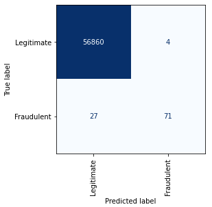
Given the credit-card fraud-detection dataset, how would you build a model around it? One way to do it is to train a supervised-learning model – a binary classifier – to predict 1s and 0s. I built one such model in a Jupyter notebook and found that a random-forest classifier yielded the best results. It detected about 75% of the fraudulent transactions while misclassifying just 4 of 56,854 legitimate transactions as fraudulent. Here is the confusion matrix:
Supervised learning isn’t the only option, however. Here’s a second notebook that uses PCA-based anomaly detection to identify fraudulent transactions. This version begins by loading the dataset, separating the samples by class into one dataset representing legitimate transactions and another representing fraudulent transactions, and dropping the Time and Class columns:
import pandas as pd

df = pd.read_csv('Data/creditcard.csv')
df.head()

# Separate the samples by class
legit = df[df['Class'] == 0]
fraud = df[df['Class'] == 1]

# Drop the "Time" and "Class" columns
legit = legit.drop(['Time', 'Class'], axis=1)
fraud = fraud.drop(['Time', 'Class'], axis=1)
It then uses PCA to reduce the two datasets from 29 to 26 dimensions, and inverts the transform to restore each dataset to 29 dimensions. Note that the transform is fitted to legitimate transactions only, but applied to both sets:
from sklearn.decomposition import PCA

pca = PCA(n_components=26, random_state=0)
legit_pca = pd.DataFrame(pca.fit_transform(legit), index=legit.index)
fraud_pca = pd.DataFrame(pca.transform(fraud), index=fraud.index)

legit_restored = pd.DataFrame(pca.inverse_transform(legit_pca), index=legit_pca.index)
fraud_restored = pd.DataFrame(pca.inverse_transform(fraud_pca), index=fraud_pca.index)
Some information was lost in the transition. Hopefully, the fraudulent transactions incurred more loss than the legitimate ones, and we can use that to differentiate between them. The next step is to compute the loss for each row in the two datasets by summing the squares of the differences between the values in the original rows and the restored rows:
import numpy as np

def get_anomaly_scores(df_original, df_restored):
    loss = np.sum((np.array(df_original) - np.array(df_restored)) ** 2, axis=1)
    loss = pd.Series(data=loss, index=df_original.index)
    return loss

legit_scores = get_anomaly_scores(legit, legit_restored)
fraud_scores = get_anomaly_scores(fraud, fraud_restored)
Plotting the losses for each dataset reveals that most of the rows in the dataset representing legitimate transactions incurred a loss of less than 200, while many of the rows in the dataset representing fraudulent transactions incurred a loss greater than 200. Separating the rows on this basis – classifying transactions with a loss of less than 200 as legitimate and transactions with a higher loss as fraudulent – produces the following confusion matrix:
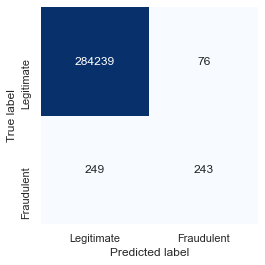
The results aren’t quite as good as they were with the random forest, but the model still caught about 50% of the fraudulent transactions while mislabeling just 76 out of 284,315 legitimate transactions. That’s an error rate of less than 0.03% for legitimate transactions, compared to 0.007% for the supervised-learning model.
Two parameters in this model drive the error rate: the number of columns the datasets were reduced to with PCA (26), and the threshold chosen to distinguish between legitimate and fraudulent transactions (200). You can tweak the accuracy by experimenting with different values. I did some informal testing and concluded that this was a reasonable combination. Picking a lower threshold improves the model’s ability to identify fraudulent transactions, but at the cost of misclassifying more legitimate transactions. In the end, you have to decide what error rate you’re willing to live with, keeping in mind that declining a legitimate credit-card purchase is likely to create an unhappy customer.
Using PCA to Predict Bearing Failure
One of the classic uses for anomaly detection is to predict failures in rotating machinery. Let’s apply PCA-based anomaly detection to a subset of a dataset published by NASA to predict failures in bearings. The dataset contains vibration data for four bearings supporting a rotating shaft with a radial load of 6,000 pounds applied to it. The bearings were run to failure, and vibration data was captured by PCB 353B33 high-sensitivity quartz accelerometers at regular intervals until failure occurred.
First, download the CSV file containing the subset I culled from the larger NASA dataset. Then create a Jupyter notebook and load the data:
import pandas as pd

df = pd.read_csv('Data/bearings.csv', index_col=0, parse_dates=[0])
df.head()
The dataset contains 984 samples. Each sample contains vibration data for four bearings, and the samples were taken 10 minutes apart. Plot the vibration data for all four bearings as a time series:
import matplotlib.pyplot as plt
%matplotlib inline
import seaborn as sns
sns.set()

df.plot(figsize = (12, 6))
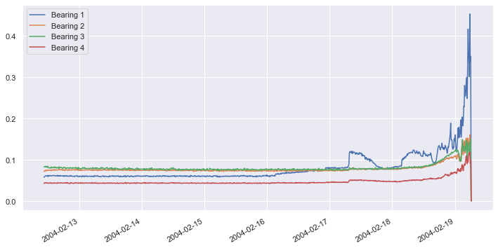
About four days into the test, vibrations in bearing #1 began increasing. They spiked a day later, and about two days after that, bearing #1 suffered a catastrophic failure. Our goal is to build a model that recognizes increased vibration in any bearing as a sign of impending failure, and to do it without a labeled dataset.
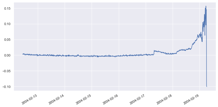
The next step is to extract samples representing “normal” operation from the dataset, and reduce four dimensions to one using PCA – essentially combining the data from all four bearings so we can monitor them as a group. Then apply the same PCA transform to the remainder of the dataset, invert the transform, and plot the reconstructed dataset to visualize the loss. Start by reducing the dataset to one dimension with PCA and plotting the result:
from sklearn.decomposition import PCA

x_train = df['2004-02-12 10:32:39':'2004-02-13 23:42:39']
x_test = df['2004-02-13 23:52:39':]

pca = PCA(n_components=1, random_state=0)
x_train_pca = pd.DataFrame(pca.fit_transform(x_train))
x_train_pca.index = x_train.index

x_test_pca = pd.DataFrame(pca.transform(x_test))
x_test_pca.index = x_test.index

df_pca = pd.concat([x_train_pca, x_test_pca])
df_pca.plot(figsize = (12, 6))
plt.legend().remove()
Now invert the PCA transform and plot the “restored” dataset:
df_restored = pd.DataFrame(pca.inverse_transform(df_pca), index=df_pca.index)
df_restored.plot(figsize = (12, 6))
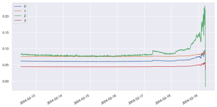
It is obvious that loss was incurred by applying and inverting the transform. Let’s define a function that computes the loss in a range of samples. Then apply that function to all of the samples in the original dataset and the restored dataset and plot the differences over time:
import numpy as np

def get_anomaly_scores(df_original, df_restored):
    loss = np.sum((np.array(df_original) - np.array(df_restored)) ** 2, axis=1)
    loss = pd.Series(data=loss, index=df_original.index)
    return loss

scores = get_anomaly_scores(df, df_restored)
scores.plot(figsize = (12, 6))
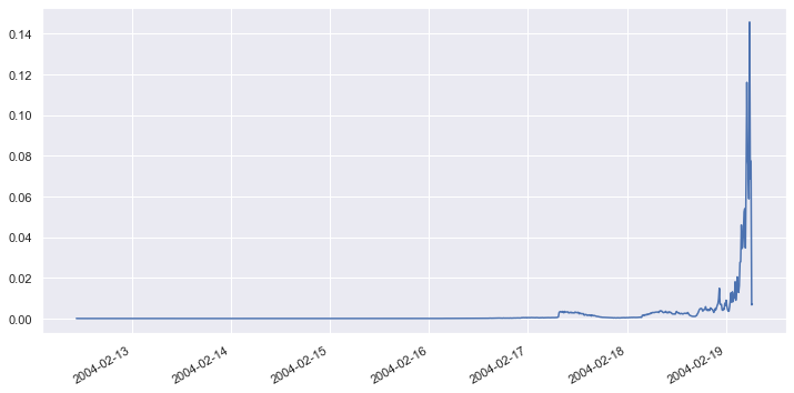
The loss is very small when all four bearings are operating normally, but it begins to rise when one or more bearings exhibits greater-than-normal vibration. From the chart, it’s apparent that when the loss rises above a threshold value of approximately 0.002, that’s an indication that a bearing might fail.
Now that we’ve selected a tentative loss threshold, we can use it to detect anomalous behavior in the bearing set. Begin by defining a function that takes a sample as input and returns True or False indicating whether the sample is anomalous by applying and inverting a PCA transform, measuring the loss, and comparing it to a specified loss threshold:
def is_anomaly(data, pca, threshold):
    pca_data = pca.transform(data)
    restored_data = pca.inverse_transform(pca_data)
    loss = np.sum((data - restored_data) ** 2)
    return loss > threshold
Apply the function to a row early in the time series that represents normal behavior:
x = [df.loc['2004-02-16 22:52:39']]
is_anomaly(x, pca, 0.002)
Apply the function to a row later in the time series that represents anomalous behavior:
x = [df.loc['2004-02-18 22:52:39']]
is_anomaly(x, pca, 0.002)
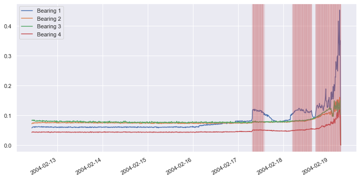
Now apply the function to all the samples in the dataset and shade anomalous samples red in order to visualize when anomalous behavior is detected:
df.plot(figsize = (12, 6))

for index, row in df.iterrows():
    if is_anomaly([row], pca, 0.002):
        plt.axvline(row.name, color='r', alpha=0.2)
Repeat this procedure, but this time use a loss threshold of 0.0002 rather than 0.002 to detect anomalous behavior:
df.plot(figsize = (12, 6))

for index, row in df.iterrows():
    if is_anomaly([row], pca, 0.0002):
        plt.axvline(row.name, color='r', alpha=0.2)
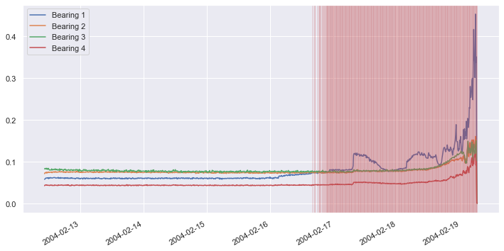
You can adjust the sensitivity of the model by adjusting the threshold value used to detect anomalies. Using a loss threshold of 0.002 predicts bearing failure about two days before it occurs, while a loss threshold of 0.0002 predicts the failure about three days before. You typically want to choose a loss threshold that predicts failure as early as possible without raising false alarms.
Get the Code
You can download a Jupyter notebook containing the bearing-failure example from the machine-learning repo that I maintain on GitHub. Feel free to check out the other notebooks in the repo while you’re at it. Also be sure to check back from time to time because I am constantly uploading new samples and updating existing ones.
