My previous post demonstrated how to use transfer learning to build a model that with just 300 training images can classify photos of three different types of Arctic wildlife with 95% accuracy. One of the benefits of transfer learning is that it can do a lot with relatively few images. This feature, however, can also be a bug. With just 100 or samples of each class, there isn’t a lot of diversity among images. A model might be able to recognize a polar bear if the bear’s head is perfectly aligned in center of the photo. But if the training images don’t include photos with the bear’s head aligned differently or tilted at different angles, the model might have difficulty classifying the photo.
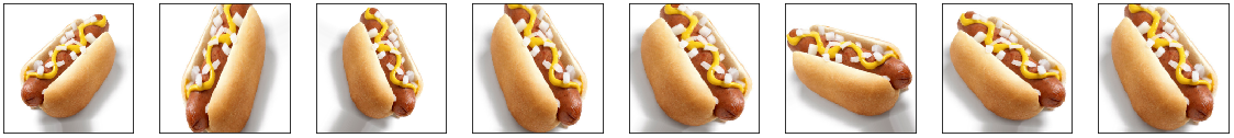
One solution is data augmentation. Rather than scare up more training images, you can rotate, translate, and scale the images you have. It doesn’t always increase accuracy, but it frequently does. Keras makes it easy to randomly transform training images provided to a network. Images are transformed differently in each epoch, so if you train for 10 epochs, the network sees 10 different variations of each training image. This can increase a model’s ability to generalize with little to no impact on training time. The figure below shows the effect of applying random transforms to a hot-dog image. You can see why presenting the same image to a model in different ways might make the model more adept at recognizing hot dogs, regardless of how the hot dog is framed.
Keras has built-in support for data augmentation with images. Let’s look at a couple of ways to put image augmentation to work, and then apply it to the Arctic-wildlife model presented in the previous post.
Image Augmentation with ImageDataGenerator
One way to leverage image augmentation when training a model is to use Keras’s ImageDataGenerator class. ImageDataGenerator generates batches of training images on the fly, either from images you’ve loaded (for example, with Keras’s load_img function) or from a specified location in the file system. The latter is especially useful when training CNNs with millions of images because it loads images into memory in batches rather than all at once. Regardless of where the images come from, however, ImageDataGenerator is happy to apply transforms as it serves them up.
Here’s a simple example that you can try yourself. Use the following code to load an image from your file system, wrap an ImageDataGenerator around it, and generate 24 versions of the image. Be sure to replace polar_bear.png on line 8 with the path to the image:
import numpy as np
from keras.preprocessing import image
from tensorflow.keras.preprocessing.image import ImageDataGenerator
import matplotlib.pyplot as plt
%matplotlib inline

# Load an image
x = image.load_img('polar_bear.png')
x = image.img_to_array(x)
x = np.expand_dims(x, axis=0)

# Wrap an ImageDataGenerator around it
idg = ImageDataGenerator(rescale=1./255,
                         horizontal_flip=True,
                         rotation_range=30,
                         width_shift_range=0.2,
                         height_shift_range=0.2,
                         zoom_range=0.2)
idg.fit(x)

# Generate 24 versions of the image
generator = idg.flow(x, [0], batch_size=1, seed=0)
fig, axes = plt.subplots(3, 8, figsize=(16, 6), subplot_kw={'xticks': [], 'yticks': []})

for i, ax in enumerate(axes.flat):
    img, label = generator.next()
    ax.imshow(img[0])
Here’s the result:
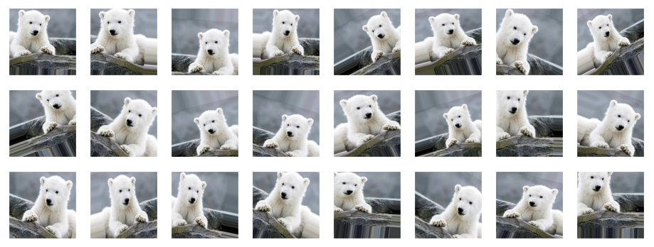
The parameters passed to ImageDataGenerator tell it how to transform the image each time it’s fetched:
- rescale=1./255 divides each pixel value by 255
- horizontal_flip=True randomly flips the image horizontally (around a vertical axis)
- rotation_range=30 randomly rotates the image by -30 to 30 degrees
- width_shift_range=0.2 and height_shift_range=0.2 randomly translate the image by -20% to 20%
- zoom_range=0.2 randomly scales the image by -20% to 20%
There are other parameters that you can use such as vertical_flip, shear_range, and brightness_range, but you get the picture. The flow method generates images from the images you pass to fit. The related flow_from_directory method loads images from the file system and optionally labels them based on the subdirectories they’re in.
The generator returned by flow can be passed directly to a model’s fit method to provide randomly transformed images to the model as it is trained. Assume that x_train and y_train hold a collection of training images and labels. The following code wraps an ImageDataGenerator around them and uses them to train a model:
idg = ImageDataGenerator(rescale=1./255,
                         horizontal_flip=True,
                         rotation_range=30,
                         width_shift_range=0.2,
                         height_shift_range=0.2,
                         zoom_range=0.2)

idg.fit(x_train)
image_batch_size = 10
generator = idg.flow(x_train, y_train, batch_size=image_batch_size, seed=0)

model.fit(generator,
          steps_per_epoch=len(x_train) // image_batch_size,
          validation_data=(x_test, y_test),
          batch_size=20,
          epochs=10)
The steps_per_epoch parameter is key because an ImageDataGenerator can provide an infinite number of versions of each image. In this example, the batch_size parameter passed to flow tells the generator to create 10 images in each batch (each call to next). Dividing the number of images by the image batch size to calculate steps_per_epoch ensures that in each training epoch, the model is provided with one transformed version of each image in the dataset.
Observe that the call to fit includes a validation_data parameter identifying a separate set of images and labels for validating the network during training. You generally don’t want to augment validation images, so you should avoid using validation_split when passing a generator to fit.
Image Augmentation with Augmentation Layers
You can use ImageDataGenerator to provide transformed images to a model, but recent versions of Keras provide an alternative in the form of image-preprocessing layers and image-augmentation layers. Rather than transform training images separately, you can integrate the transforms into the model. Here’s an example:
from keras.models import Sequential
from keras.layers import Conv2D, MaxPooling2D
from keras.layers import Rescaling, RandomFlip, RandomRotation, RandomTranslation, RandomZoom
from keras.layers import Flatten, Dense

model = Sequential()
model.add(Rescaling(1./255))
model.add(RandomFlip(mode='horizontal'))
model.add(RandomTranslation(0.2, 0.2))
model.add(RandomRotation(0.2))
model.add(RandomZoom(0.2))
model.add(Conv2D(32, (3, 3), activation='relu', input_shape=(224, 224, 3)))
model.add(MaxPooling2D(2, 2))
model.add(Conv2D(128, (3, 3), activation='relu'))
model.add(MaxPooling2D(2, 2))
model.add(Flatten())
model.add(Dense(128, activation='relu'))
model.add(Dense(3, activation='softmax')
Each image used to train the CNN has its pixel values divided by 255 and is then randomly flipped, translated, rotated, and scaled. Significantly, the RandomFlip, RandomTranslation, RandomRotation, and RandomZoom layers only operate on training images. They are inactive when the network is validated or asked to make predictions. The Rescaling layer is active at all times, meaning you no longer have to remember to divide by 255 before passing an image to the network for classification.
Apply Image Augmentation to Arctic Wildlife
Would image augmentation make the model featured in my previous post even better? There’s one way to find out.
If you haven’t already, download the zip file containing wildlife images. Unpack the zip file and place its contents in the directory where your Jupyter notebooks are hosted. The zip file contains folders named “train,” “test,” and “samples.” Each folder contains subfolders named “arctic_fox,” “polar_bear,” and “walrus.” The training folders contain 100 images each, while the test folders contain 40 images each.
Create a Jupyter notebook and paste the following code into the first cell to define helper functions for loading and labeling images and declare Python lists for accumulating images and labels:
import os
import numpy as np
from keras.preprocessing import image
import matplotlib.pyplot as plt
%matplotlib inline

def load_images_from_path(path, label):
    images = []
    labels = []

    for file in os.listdir(path):
        img = image.load_img(os.path.join(path, file), target_size=(224, 224, 3))
        images.append(image.img_to_array(img))
        labels.append((label))

    return images, labels

def show_images(images):
    fig, axes = plt.subplots(1, 8, figsize=(20, 20), subplot_kw={'xticks': [], 'yticks': []})

    for i, ax in enumerate(axes.flat):
        ax.imshow(images[i] / 255)

x_train = []
y_train = []
x_test = []
y_test = []
Use the following statements to load the Arctic-fox training images and plot a few of them:
images, labels = load_images_from_path('train/arctic_fox', 0)
show_images(images)

x_train += images
y_train += labels
Load and label the polar-bear training images:
images, labels = load_images_from_path('train/polar_bear', 1)
show_images(images)

x_train += images
y_train += labels
And then the walrus training images:
images, labels = load_images_from_path('train/walrus', 2)
show_images(images)

x_train += images
y_train += labels
The dataset also contains test images. Load the Arctic-fox test images:
images, labels = load_images_from_path('test/arctic_fox', 0)
show_images(images)

x_test += images
y_test += labels
Then the polar-bear test images:
images, labels = load_images_from_path('test/polar_bear', 1)
show_images(images)

x_test += images
y_test += labels
And finally, the walrus test images:
images, labels = load_images_from_path('test/walrus', 2)
show_images(images)

x_test += images
y_test += labels
The next step is to one-hot-encode the labels and preprocess the images the way ResNet50V2 expects. Note that there is no need to divide pixel values by 255 because we’ll include a Rescaling layer in our network to do that:
from tensorflow.keras.utils import to_categorical
from tensorflow.keras.applications.resnet50 import preprocess_input

x_train = preprocess_input(np.array(x_train))
x_test = preprocess_input(np.array(x_test))

y_train_encoded = to_categorical(y_train)
y_test_encoded = to_categorical(y_test)
Now load ResNet50V2 without the classification layers and initialize it with the weights arrived at when it was trained on the ImageNet dataset. A key element here is preventing the bottleneck layers from training when the network is trained by setting their trainable attributes to False, effectively freezing those layers:
from tensorflow.keras.applications import ResNet50V2

base_model = ResNet50V2(weights='imagenet', include_top=False)

for layer in base_model.layers:
    layer.trainable = False
Define a network that incorporates rescaling and augmentation layers, ResNet50V2‘s bottleneck layers, dense layers for classification, and a dropout layer to help the network generalize. Then train the network using an increased number of epochs so it sees more randomly transformed training samples:
from keras.models import Sequential
from keras.layers import Flatten, Dense, Dropout
from keras.layers import Rescaling, RandomFlip, RandomRotation, RandomTranslation, RandomZoom

model = Sequential()
model.add(Rescaling(1./255))
model.add(RandomFlip(mode='horizontal'))
model.add(RandomTranslation(0.2, 0.2))
model.add(RandomRotation(0.2))
model.add(RandomZoom(0.2))
model.add(base_model)
model.add(Flatten())
model.add(Dense(1024, activation='relu'))
model.add(Dropout(0.2))
model.add(Dense(3, activation='softmax'))
model.compile(optimizer='adam', loss='categorical_crossentropy', metrics=['accuracy'])

hist = model.fit(x_train, y_train_encoded, validation_data=(x_test, y_test_encoded), batch_size=10, epochs=25)
How well did the network train? Let’s plot the training accuracy and validation accuracy for each epoch:
acc = hist.history['accuracy']
val_acc = hist.history['val_accuracy']
epochs = range(1, len(acc) + 1)

plt.plot(epochs, acc, '-', label='Training Accuracy')
plt.plot(epochs, val_acc, ':', label='Validation Accuracy')
plt.title('Training and Validation Accuracy')
plt.xlabel('Epoch')
plt.ylabel('Accuracy')
plt.legend(loc='lower right')
plt.plot()
With a little luck, the network achieved 97% to 98% accuracy, which is a couple percentage points more than it achieved without data augmentation. Use a confusion matrix to visualize how well the network performed during testing:
from sklearn.metrics import confusion_matrix
import seaborn as sns
sns.set()

y_predicted = model.predict(x_test)
mat = confusion_matrix(y_test_encoded.argmax(axis=1), y_predicted.argmax(axis=1))
class_labels = ['arctic fox', 'polar bear', 'walrus']

sns.heatmap(mat, square=True, annot=True, fmt='d', cbar=False, cmap='Blues',
            xticklabels=class_labels,
            yticklabels=class_labels)

plt.xlabel('Predicted label')
plt.ylabel('Actual label')
Use the following statements to load an Arctic-fox image that the network was neither trained nor tested with:
x = image.load_img('samples/arctic_fox/arctic_fox_140.jpeg', target_size=(224, 224))
plt.xticks([])
plt.yticks([])
plt.imshow(x)
Preprocess the image and see how the network classifies it:
x = image.img_to_array(x)
x = np.expand_dims(x, axis=0)
x = preprocess_input(x)
predictions = model.predict(x)

for i, label in enumerate(class_labels):
    print(f'{label}: {predictions[0][i]}')
Now load a walrus image:
x = image.load_img('samples/walrus/walrus_143.png', target_size=(224, 224))
plt.xticks([])
plt.yticks([])
plt.imshow(x)
And submit it to the network for classification:
x = image.img_to_array(x)
x = np.expand_dims(x, axis=0)
x = preprocess_input(x)
predictions = model.predict(x)

for i, label in enumerate(class_labels):
    print(f'{label}: {predictions[0][i]}')
Data scientists often employ data augmentation even when they’re training a CNN from scratch rather than employing transfer learning. It’s a useful tool to know about, and one that could make a difference when you’re trying to squeeze every last ounce of accuracy out of a deep-learning model.
Get the Code
You can download a Jupyter notebook demonstrating transfer learning with data augmentation from the deep-learning repo that I maintain on GitHub. Feel free to check out the other notebooks in the repo while you’re at it. Also be sure to check back from time to time because I am constantly uploading new samples and updating existing ones.
