You are the leader of a group of climate scientists concerned about the planet’s dwindling rainforests. The world loses up to 10 million acres of old-growth rainforests each year, much of it due to illegal logging. Your team plans to convert thousands of discarded smart phones into solar-powered listening devices and position them throughout the Amazon to transmit alerts in response to the sounds of chainsaws and truck engines. You need software for these phones that uses AI to identify such sounds in real time. And you need it fast, because climate change won’t wait.
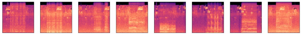
One way to perform audio classification is to convert audio streams into spectrogram images, which provide visual representations of spectrums of frequencies as they vary over time, and use convolutional neural networks (CNNs) to classify the spectrograms. The spectrograms below were generated from WAV files containing chainsaw sounds. Let’s use Keras and transfer learning to build a model that can identify the tell-tale sounds of logging operations and distinguish them from ambient sounds such as wildlife and thunderstorms.
This post was inspired by the Rainforest Connection, which uses recycled Android phones and a TensorFlow model to monitor rainforests for sounds indicative of illegal activity. For more information, see The fight against illegal deforestation with TensorFlow in the Google AI blog. It is just one example of how AI is making the world a better place.
Save the Rainforest!
Begin by downloading a dataset containing rainforest sounds. (Warning: It’s a 666 MB download.) Open the zip file and copy the “Sounds” folder into the directory where your Jupyter notebooks are hosted. “Sounds” contains subdirectories named “background,” “chainsaw,” “engine,” and “storm.” Each subdirectory contains 100 WAV files. The WAV files in the “background” directory contain rainforest background noises only, while the files in the other subdirectories include the sounds of chainsaws, engines, and thunderstorms overlaid on the background noises. These files were generated by using a soundscape-synthesis package named Scaper to combine sounds in the public UrbanSound8K dataset with rainforest sounds obtained from YouTube. Play a few of the WAV files on your computer to get an idea of the sounds they contain.
Now create a Jupyter notebook and paste following code into the first cell:
import numpy as np
import librosa.display, os
import matplotlib.pyplot as plt
%matplotlib inline

def create_spectrogram(audio_file, image_file):
    fig = plt.figure()
    ax = fig.add_subplot(1, 1, 1)
    fig.subplots_adjust(left=0, right=1, bottom=0, top=1)

    y, sr = librosa.load(audio_file)
    ms = librosa.feature.melspectrogram(y, sr=sr)
    log_ms = librosa.power_to_db(ms, ref=np.max)
    librosa.display.specshow(log_ms, sr=sr)

    fig.savefig(image_file)
    plt.close(fig)

def create_pngs_from_wavs(input_path, output_path):
    if not os.path.exists(output_path):
        os.makedirs(output_path)

    dir = os.listdir(input_path)

    for i, file in enumerate(dir):
        input_file = os.path.join(input_path, file)
        output_file = os.path.join(output_path, file.replace('.wav', '.png'))
        create_spectrogram(input_file, output_file)
This code defines a pair of functions to help convert WAV files into spectrogram images. create_spectrogram uses a Python package named Librosa to create a spectrogram image from a WAV file. create_pngs_from_wavs converts all the WAV files in a specified directory into spectrogram images. You will need to install Librosa if it isn’t installed already.
Use the following statements to create PNG files containing spectrograms from all the WAV files in the “Sounds” directory’s subdirectories:
create_pngs_from_wavs('Sounds/background', 'Spectrograms/background')
create_pngs_from_wavs('Sounds/chainsaw', 'Spectrograms/chainsaw')
create_pngs_from_wavs('Sounds/engine', 'Spectrograms/engine')
create_pngs_from_wavs('Sounds/storm', 'Spectrograms/storm')
Check the “Spectrograms” directory for subdirectories containing spectrograms and confirm that each subdirectory contains 100 PNG files. Then use the following code to define two new helper functions for loading and displaying spectrograms and to declare two Python lists — one to store spectrogram images, and another to store class labels:
from keras.preprocessing import image

def load_images_from_path(path, label):
    images = []
    labels = []

    for file in os.listdir(path):
        images.append(image.img_to_array(image.load_img(os.path.join(path, file), target_size=(224, 224, 3))))
        labels.append((label))

    return images, labels

def show_images(images):
    fig, axes = plt.subplots(1, 8, figsize=(20, 20), subplot_kw={'xticks': [], 'yticks': []})

    for i, ax in enumerate(axes.flat):
        ax.imshow(images[i] / 255)

x = []
y = []
Use the following statements to load the background spectrogram images, add them to the list named x, and label them with 0s:
images, labels = load_images_from_path('Spectrograms/background', 0)
show_images(images)

x += images
y += labels
Repeat this process to load chainsaw spectrograms from the “Spectrograms/chainsaw” directory, engine spectrograms from the “Spectrograms/engine” directory, and thunderstorm spectrograms from the “Spectrograms/storm” directory. Label chainsaw images with 1s, engine spectrograms with 2s, and thunderstorm spectrograms with 3s. Here is a summary of the class labels used for the four classes of images:
| Spectrogram Type | Label |
|---|---|
| background | 0 |
| chainsaw | 1 |
| engine | 2 |
| storm | 3 |
Now use the following code to split the images and labels into two datasets — one for training, and one for testing — and also to divide the pixel values by 255 and one-hot-encode the labels using Keras’s to_categorical function:
from tensorflow.keras.utils import to_categorical
from sklearn.model_selection import train_test_split

x_train, x_test, y_train, y_test = train_test_split(x, y, stratify=y, test_size=0.3, random_state=0)

x_train_norm = np.array(x_train) / 255
x_test_norm = np.array(x_test) / 255

y_train_encoded = to_categorical(y_train)
y_test_encoded = to_categorical(y_test)
Transfer learning is a powerful technique that allows sophisticated CNNs trained by Google, Microsoft, and others on GPUs to be repurposed and used to solve domain-specific problems. Many pretrained CNNs are available in the public domain, and several are included with Keras. Let’s use MobileNetV2, a pretrained CNN from Google that is optimized for mobile devices, to extract features from spectrogram images.
Start by calling Keras’s MobileNetV2 function to instantiate MobileNetV2 without the classification layers. Use the preprocess_input function for MobileNet networks to preprocess the training and testing images. Then run both datasets through MobileNetV2 to extract features:
from tensorflow.keras.applications import MobileNetV2
from tensorflow.keras.applications.mobilenet import preprocess_input

base_model = MobileNetV2(weights='imagenet', include_top=False, input_shape=(224, 224, 3))

x_train_norm = preprocess_input(np.array(x_train))
x_test_norm = preprocess_input(np.array(x_test))

train_features = base_model.predict(x_train_norm)
test_features = base_model.predict(x_test_norm)
Define a neural network to classify features extracted by MobileNetV2‘s bottleneck layers:
model = Sequential()
model.add(Flatten(input_shape=train_features.shape[1:]))
model.add(Dense(1024, activation='relu'))
model.add(Dense(4, activation='softmax'))
model.compile(optimizer='adam', loss='categorical_crossentropy', metrics=['accuracy'])
Train the network with the features:
hist = model.fit(train_features, y_train_encoded, validation_data=(test_features, y_test_encoded), batch_size=10, epochs=10)
Plot the training and validation accuracy:
acc = hist.history['accuracy']
val_acc = hist.history['val_accuracy']
epochs = range(1, len(acc) + 1)

plt.plot(epochs, acc, '-', label='Training Accuracy')
plt.plot(epochs, val_acc, ':', label='Validation Accuracy')
plt.title('Training and Validation Accuracy')
plt.xlabel('Epoch')
plt.ylabel('Accuracy')
plt.legend(loc='lower right')
plt.plot()
Run the test images through the network and use a confusion matrix to assess the results:
from sklearn.metrics import confusion_matrix
import seaborn as sns
sns.set()

y_predicted = model.predict(test_features)
mat = confusion_matrix(y_test_encoded.argmax(axis=1), y_predicted.argmax(axis=1))
class_labels = ['background', 'chainsaw', 'engine', 'storm']

sns.heatmap(mat, square=True, annot=True, fmt='d', cbar=False, cmap='Blues',
            xticklabels=class_labels,
            yticklabels=class_labels)

plt.xlabel('Predicted label')
plt.ylabel('Actual label')
The network is pretty adept at identifying clips that don’t contain the sounds of chainsaws or engines. It sometimes confuses chainsaw sounds and engine sounds, but that’s OK, because the presence of either might indicate illicit activity in a rainforest.
Test with Unrelated WAV Files
The “Sounds” directory has a subdirectory named “samples” containing WAV files that the CNN was neither trained nor tested with. The WAV files bear no relation to the samples used for training and testing; they were extracted from a YouTube video documenting Brazil’s efforts to curb illegal logging. Let’s use the model you just trained to analyze these files for sounds of logging activity.
Start by creating a spectrogram from the first sample WAV file, which contains audio of loggers cutting down trees in the Amazon:
create_spectrogram('Sounds/samples/sample1.wav', 'Spectrograms/sample1.png')

x = image.load_img('Spectrograms/sample1.png', target_size=(224, 224))
plt.xticks([])
plt.yticks([])
plt.imshow(x)
Preprocess the spectrogram image, pass it to MobileNetV2 for feature extraction, and classify the features:
x = image.img_to_array(x)
x = np.expand_dims(x, axis=0)
x = preprocess_input(x)

y = base_model.predict(x)
predictions = model.predict(y)

for i, label in enumerate(class_labels):
    print(f'{label}: {predictions[0][i]}')
Create a spectrogram from a WAV file that includes the sounds of a logging truck rumbling through the rainforest:
create_spectrogram('Sounds/samples/sample2.wav', 'Spectrograms/sample2.png')

x = image.load_img('Spectrograms/sample2.png', target_size=(224, 224))
plt.xticks([])
plt.yticks([])
plt.imshow(x)
Preprocess the spectrogram image, pass it to MobileNetV2 for feature extraction, and classify the features:
x = image.img_to_array(x)
x = np.expand_dims(x, axis=0)
x = preprocess_input(x)

y = base_model.predict(x)
predictions = model.predict(y)

for i, label in enumerate(class_labels):
    print(f'{label}: {predictions[0][i]}')
If the network got either of the samples wrong, try training it again. Remember that a neural network will train differently every time, in part because Keras initializes the weights with small random values. In the real world, data scientists often train a neural network several times and average the results to quantify its accuracy.
Get the Code
You can download a Jupyter notebook containing the audio-classification example from the deep-learning repo that I maintain on GitHub. Feel free to check out the other notebooks in the repo while you’re at it. Also be sure to check back from time to time because I am constantly uploading new samples and updating existing ones.
