Computer vision is a branch of AI in which computers extract perceptual information from images. Real-world uses include identifying objects in photos, removing inappropriate images from social-media sites, flagging defective parts coming off an assembly line, and facial recognition. Computer-vision models can even be combined with natural language processing (NLP) models to caption photos. I snapped a photo on vacation last summer and asked Azure’s Computer Vision service to caption it. The result is shown below. It’s pretty remarkable given that no human intervention was required.
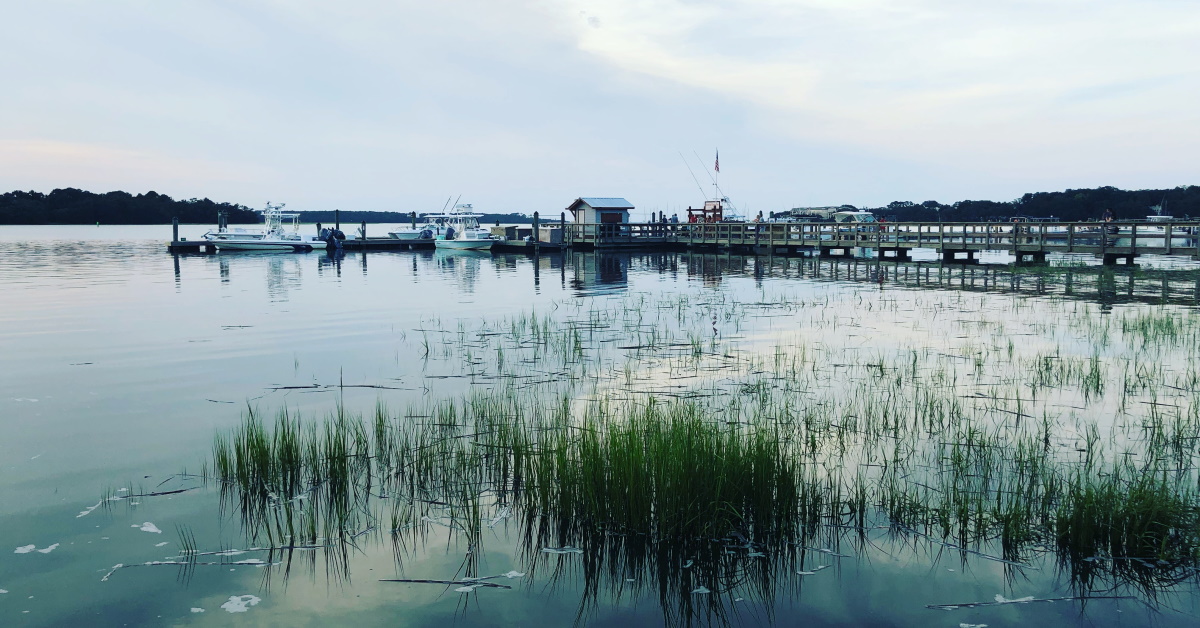
“A body of water with a dock and a building in the background” — Azure AI
The field of computer vision has advanced rapidly in recent years, mostly due to convolutional neural networks, or CNNs. In 2012, an 8-layer CNN called AlexNet outperformed traditional machine-learning models entered in the annual ImageNet Large Scale Visual Recognition Challenge (ILSVRC) by achieving an error rate of 15.3% identifying objects in photos. In 2015, Microsoft’s ResNet-152 CNN featuring a whopping 152 layers won the challenge with an error rate of just 3.5%, which exceeds a human’s ability to classify images used in the competition.
CNNs are magical because they treat images as images rather than just arrays of numbers. They use a decades-old technology called convolution kernels to extract “features” from images, allowing them to recognize the shape of a cat’s head or the outline of a dog’s tail. Moreover, they are easy to build with Keras and TensorFlow.
State-of-the-art CNNs such as ResNet-152 are trained at great expense with millions of images on cloud-based GPU clusters, but there’s still a lot that you can do with a single GPU or an ordinary CPU. In this post, you’ll learn what CNNs are and how they work, and you’ll build and train your first CNN. In subsequent posts, you’ll learn how to leverage advanced CNNs published for public consumption by companies such as Google and Microsoft, as well as how to use a technique called transfer learning to repurpose those CNNs to solve domain-specific problems.
Understanding CNNs
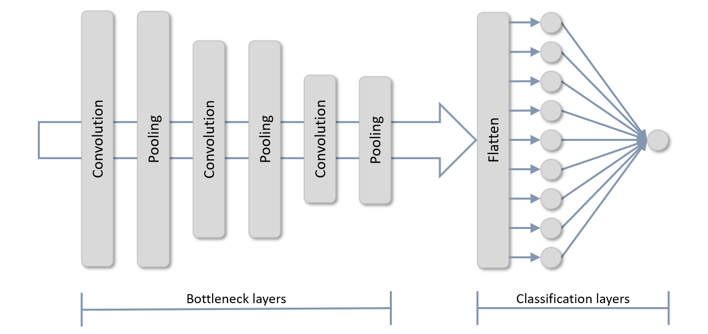
The diagram below shows the topology of a typical CNN. It begins with one or more pairs of convolution layers and pooling layers. Convolution layers extract features from images; pooling layers reduce the images’ size, typically by half, so features can be extracted at various resolutions and are less sensitive to small changes in position. Output from the final pooling layer is flattened to one dimension and input to one or more dense layers for classification. In this example, the output layer contains a single neuron designed to do binary classification. The convolution and pooling layers are sometimes referred to as bottleneck layers since they reduce the dimensionality of images passed through the pipeline. They also account for the bulk of the computation time during training.
Convolution layers extract features from images by passing convolution kernels over them – the same technique used by image-editing tools to blur, sharpen, and emboss images. A kernel is simply a matrix of values. It usually measures 3 x 3, but can be larger. To process an image, you place the kernel in the upper-left corner of the image, multiply the kernel values by the pixel values underneath, and replace the center pixel with the sum of the products. Then you move the kernel one pixel to the right and repeat the process, continuing row by row until every pixel in the image has been transformed.
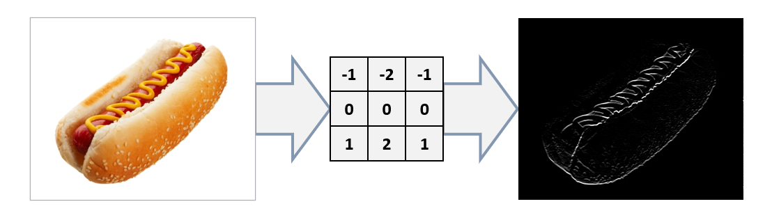
The figure below shows what happens when you apply a 3 x 3 kernel to a hot-dog image. This particular kernel is called a bottom Sobel kernel, and it’s designed to do edge detection by highlighting edges as if a light were shined from the bottom. The convolution layers of a CNN use kernels like this one to examine images from various angles and highlight features that might help distinguish one class from another.
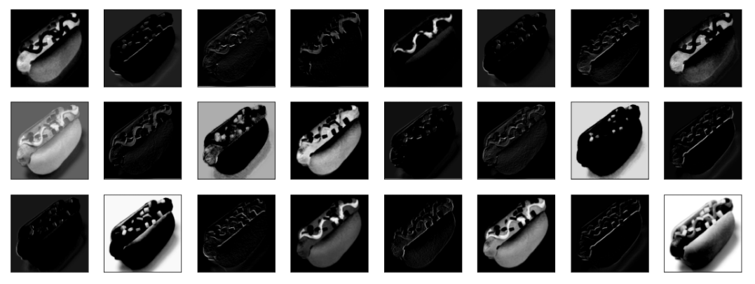
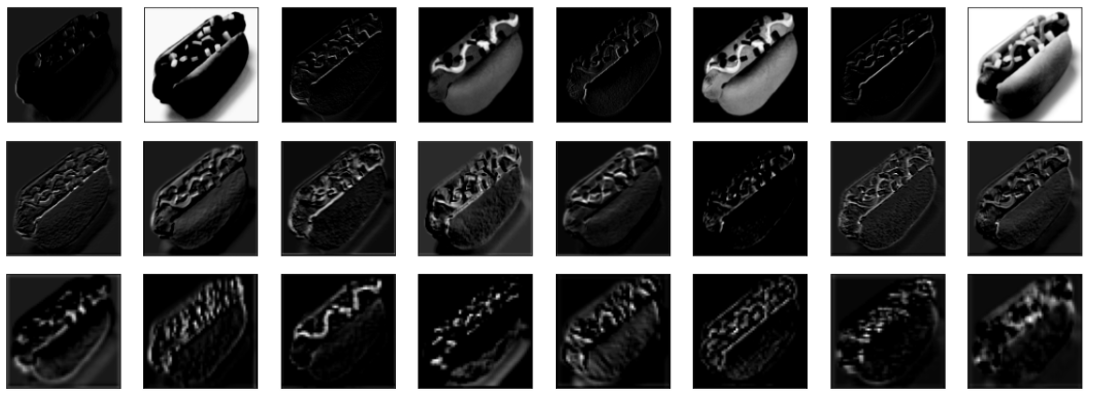
A convolution layer doesn’t use just one kernel to process images. It uses several – sometimes 100 or more. The kernel values aren’t fixed. They are initialized with random values, and then learned (adjusted) as the CNN is trained, just as the weights connecting neurons in dense layers are learned. The images below were generated by the first convolution layer in a trained CNN. You can see how the various convolution kernels allow the network to view the same hot-dog image in different ways, and how certain features such as the shape of the bun and the ribbon of mustard on top are highlighted.
Pooling layers downsample images to reduce their size. The most common downsampling technique is max pooling, which divides images into 2 x 2 blocks of pixels and chooses the highest of the four values in each block. An alternative is average pooling, which averages the values in each block. The images below show how the resolution of an image is reduced as it passes through successive pooling layers.
The dense layer (or layers) at the end and the output layer classify features extracted from the bottleneck layers and are often referred to as the CNN’s classification layers. They are no different than the multilayer perceptrons featured in previous posts. In a multiclass-classification scenario, the output layer contains one neuron per class and uses the softmax activation function.
To simplify building CNNs that classify images, Keras offers the Conv2D class, which models convolution layers, and MaxPooling2D, which implements max-pooling layers. The following statements create a CNN with two pairs of convolution and pooling layers, a flatten layer to reshape the output into a 1D array for input to a dense layer, a dense layer to classify the features extracted from the previous layers, and a softmax output layer for classification:
from keras.models import Sequential
from keras.layers import Conv2D, MaxPooling2D
from keras.layers import Flatten, Dense

model = Sequential()
model.add(Conv2D(32, (3, 3), activation='relu', input_shape=(224, 224, 3)))
model.add(MaxPooling2D(2, 2))
model.add(Conv2D(32, (3, 3), activation='relu'))
model.add(MaxPooling2D(2, 2))
model.add(Flatten())
model.add(Dense(128, activation='relu'))
model.add(Dense(3, activation='softmax'))
The first parameter passed to the Conv2D function is the number of convolution kernels that the layer should include. The second parameter is the dimensions of each kernel. You can sometimes get more accuracy from 5 x 5 kernels, but a kernel that size increases training time by requiring 25 multiplication operations for each pixel as opposed to 9 for a 3 x 3 kernel. The input_shape parameter in the first convolution layer specifies the size of the images input to the layer: in this case, 3-channel (color) 224 x 224 images. All of the images used to train a CNN must be the same size. And while it’s not a strict requirement, CNNs generally work better when the images are square.
Train a CNN to Recognize Arctic Wildlife
The best way to acquaint yourself with CNNs is to roll up your sleeves and build one. The following tutorial steps you through the process of building and training a CNN to classify images – specifically, to classify an image as one containing an Arctic fox, a polar bear, or a walrus. It’s inspired by a demo I wrote for Microsoft that uses AI to examine pictures snapped by motion-activated cameras deployed in the Arctic to show polar-bear activity on a map.
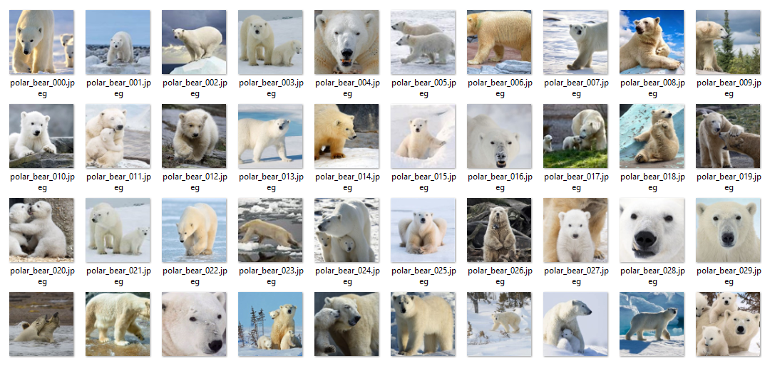
Start by downloading a zip file containing images for training the CNN. Unpack the zip file and place its contents in the directory where your Jupyter notebooks are hosted. The zip file contains folders named “train,” “test,” and “samples.” Each folder contains subfolders named “arctic_fox,” “polar_bear,” and “walrus.” The training folders contain 100 images each, while the test folders contain 40 images each. Here’s an example of some of the polar-bear training images. These images were downloaded from the Internet and cropped and resized to 224 x 224 pixels.
Now create a Jupyter notebook and use the following code to define a pair of helper functions: one to load a batch of images from a specified location in the file system and assign them labels, and another to show the first eight images in a batch of images:
import os
import numpy as np
from keras.preprocessing import image
import matplotlib.pyplot as plt
%matplotlib inline

def load_images_from_path(path, label):
    images = []
    labels = []

    for file in os.listdir(path):
        img = image.load_img(os.path.join(path, file), target_size=(224, 224, 3))
        images.append(image.img_to_array(img))
        labels.append((label))

    return images, labels

def show_images(images):
    fig, axes = plt.subplots(1, 8, figsize=(20, 20), subplot_kw={'xticks': [], 'yticks': []})

    for i, ax in enumerate(axes.flat):
        ax.imshow(images[i] / 255)

x_train = []
y_train = []
x_test = []
y_test = []
Use the following statements to load 100 Arctic-fox training images and plot a subset of them:
images, labels = load_images_from_path('train/arctic_fox', 0)
show_images(images)

x_train += images
y_train += labels
Use similar code to load and label the polar-bear training images:
images, labels = load_images_from_path('train/polar_bear', 1)
show_images(images)

x_train += images
y_train += labels
And then the walrus training images:
images, labels = load_images_from_path('train/walrus', 2)
show_images(images)

x_train += images
y_train += labels
You also need to load the images used to validate the CNN. Start with 40 Arctic-fox test images:
images, labels = load_images_from_path('test/arctic_fox', 0)
show_images(images)

x_test += images
y_test += labels
Then the polar-bear test images:
images, labels = load_images_from_path('test/polar_bear', 1)
show_images(images)

x_test += images
y_test += labels
And finally, the walrus test images:
images, labels = load_images_from_path('test/walrus', 2)
show_images(images)

x_test += images
y_test += labels
The next step is to normalize the training and testing images by dividing the pixel values by 255, and one-hot-encode the labels used for training and testing. Recall that Keras’s to_categorical function handles one-hot-encoding very nicely:
from tensorflow.keras.utils import to_categorical

x_train = np.array(x_train) / 255
x_test = np.array(x_test) / 255

y_train_encoded = to_categorical(y_train)
y_test_encoded = to_categorical(y_test)
Now it’s time to build a CNN. We’ll use four pairs of convolution and pooling layers to extract features from the training images at four resolutions: 224 x 224, 112 x 112, 56 x 56, and 28 x 28. We’ll follow those with a dense layer and a softmax output layer containing three neurons – one for each of the three classes:
from keras.models import Sequential
from keras.layers import Conv2D, MaxPooling2D
from keras.layers import Flatten, Dense

model = Sequential()
model.add(Conv2D(32, (3, 3), activation='relu', input_shape=(224, 224, 3)))
model.add(MaxPooling2D(2, 2))
model.add(Conv2D(128, (3, 3), activation='relu'))
model.add(MaxPooling2D(2, 2))
model.add(Conv2D(128, (3, 3), activation='relu'))
model.add(MaxPooling2D(2, 2))
model.add(Conv2D(128, (3, 3), activation='relu'))
model.add(MaxPooling2D(2, 2))
model.add(Flatten())
model.add(Dense(1024, activation='relu'))
model.add(Dense(3, activation='softmax'))
model.compile(optimizer='adam', loss='categorical_crossentropy', metrics=['accuracy'])
model.summary()
Call fit to train the model:
hist = model.fit(x_train, y_train_encoded, validation_data=(x_test, y_test_encoded), batch_size=10, epochs=20)
If you train the model on a CPU rather than a GPU, training will probably require from 5 to 30 seconds per epoch. When training is complete, use the following statements to plot the training and validation accuracy:
acc = hist.history['accuracy']
val_acc = hist.history['val_accuracy']
epochs = range(1, len(acc) + 1)

plt.plot(epochs, acc, '-', label='Training Accuracy')
plt.plot(epochs, val_acc, ':', label='Validation Accuracy')
plt.title('Training and Validation Accuracy')
plt.xlabel('Epoch')
plt.ylabel('Accuracy')
plt.legend(loc='lower right')
plt.plot()
Were the results what you expected? The validation accuracy is decent, but it’s not state-of-the art. It probably landed between 50% and 60%, and if you train the model several times, you’ll get different results each time. Modern CNNs often achieve an accuracy of 95% or more doing image classification. You might be able to squeeze more accuracy out of this model by adding another convolution and pooling layer or stacking convolution layers, and you might be able to get it to generalize a little better by introducing a dropout layer. But you won’t hit 95% with this network and this training set.
One of the reasons modern CNNs can do image classification so accurately is that they’re trained with millions of images. You don’t need millions of samples of each class, but you probably need at least an order of magnitude more – if not two orders of magnitude more – than the 300 you trained with here. You could scour the Internet for more images, but more images means more training time. If the goal is to achieve an accuracy of 95% or more, you’ll quickly get to the point that the CNN takes too long to train – or find yourself shopping for an NVIDIA GPU.
That doesn’t mean CNNs aren’t practical for solving business problems. It just means that there’s more to learn. Tune in next time to find out one way to attain high levels of accuracy without training a CNN from scratch.
Get the Code
You can download a Jupyter notebook containing the Arctic-wildlife example from the deep-learning repo that I maintain on GitHub. Feel free to check out the other notebooks in the repo while you’re at it. Also be sure to check back from time to time because I am constantly uploading new samples and updating existing ones.
