Deep learning is a subset of machine learning that relies primarily on neural networks. Most of what’s considered AI today is accomplished with deep learning. From recognizing objects in photos to real-time speech translation to using computers to generate art, music, poetry, and photorealistic faces, deep learning allows computers to perform feats of magic that traditional machine learning does not.
I often introduce deep learning by challenging developers to devise an algorithmic means for determining whether a photo contains a dog. You can try, but then I’ll throw out a dog picture that foils the algorithm. You can get partway there with support-vector machines, but for cognitive tasks such as object recognition, deep learning represents the state of the art. It’s not terribly difficult to train a neural network to recognize dog pictures with a high degree of accuracy – sometimes more accurately than humans. Once you learn how to do that, it’s a small step forward to recognizing defective parts coming off an assembly line or bicycles passing in front of a self-driving car.
Neural networks have been around, at least in theory, since the 1950s. But it is only in the last 10 years or so that sufficient compute power has been available to train sophisticated neural networks. Cutting-edge neural networks are trained on Graphics Processing Units (GPUs), often attached to High-Performance Computing (HPC) clusters hosted in the cloud. GPUs are great for gaming because they deliver high-performance graphics. They are also efficient parallel-processing machines that allow data scientists to train neural networks in a fraction of the time required on ordinary CPUs. Today, any researcher with a credit card can purchase an NVIDIA GPU or spin up GPUs in Azure or AWS and have access to compute power that researchers 20 years ago could only have dreamed of. This, more than anything else, has driven AI’s resurgence and led to continual advances in the state of the art.
Understanding Neural Networks
There are many kinds of neural networks. Convolutional neural networks (CNNs), for example, excel at computer-vision tasks such as identifying objects in photos. Recurrent neural networks (RNNs) find application in handwriting recognition and natural language processing (NLP), while generative adversarial networks, or GANs, enable computers to create art, music, and other content. But the first step in wrapping your head around deep learning is understanding what a neural network is and how it works.
The simplest type of neural network is the multilayer perceptron. It consists of nodes or neurons that are arranged in layers. The depth of the network is the number of layers; the width is the number of neurons in each layer. State-of-the-art neural networks sometimes contain 100 or more layers and thousands of neurons in each layer. A deep neural network is one that contains many layers, and it’s where the term deep learning derives from.
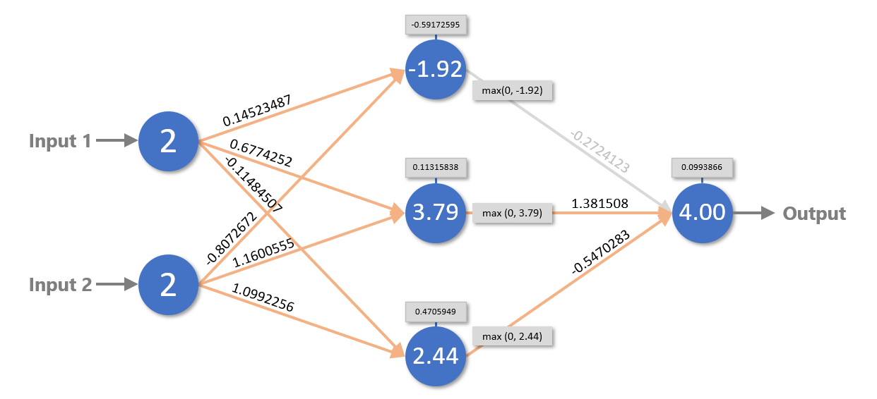
The multilayer perceptron below contains three layers: an input layer with two neurons, a middle layer (also known as a hidden layer) with three neurons, and an output layer with one neuron. This network’s job is to take two floating-point values as input and transform them to produce a single floating-point number as output. Neural networks work with floating-point numbers. They only work with floating-point numbers. As with conventional machine-learning models, a neural network can only process non-numeric data – for example, text strings – if the data is first converted to numbers.
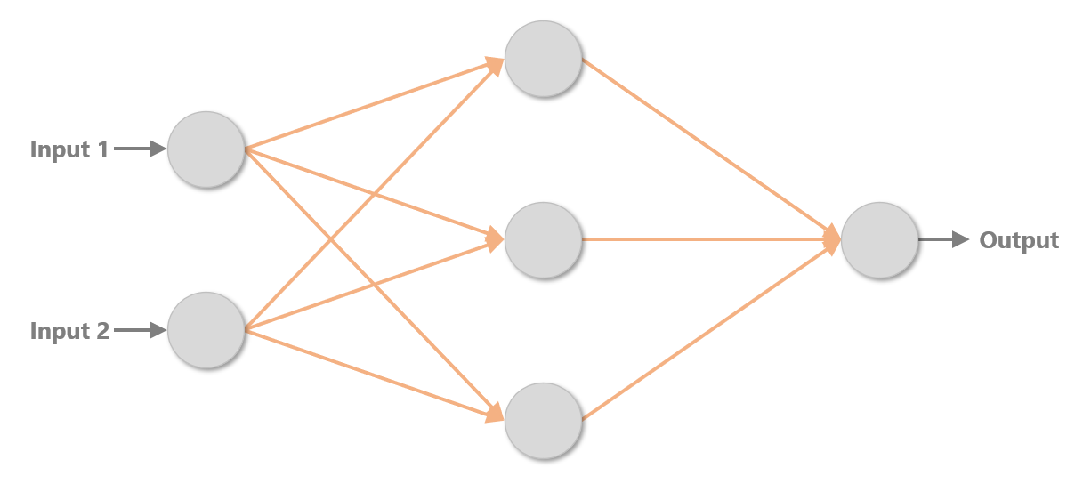
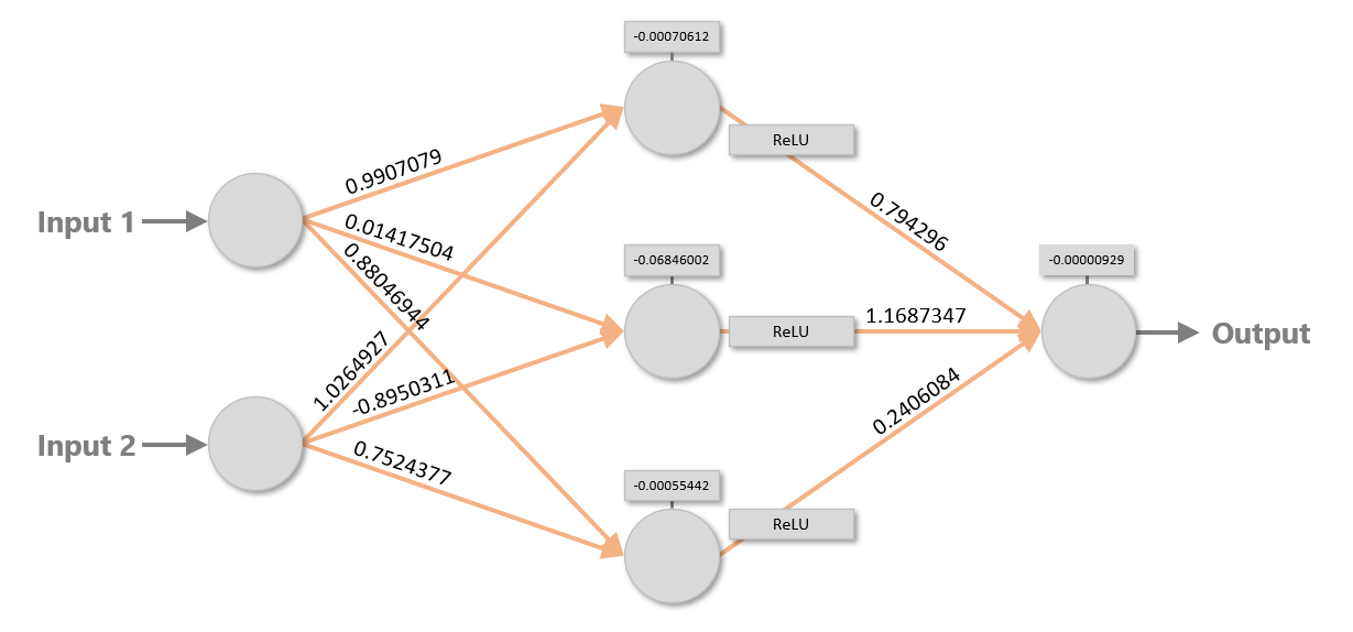
The orange arrows in the diagram represent connections between neurons. Each neuron in each layer is connected to each neuron in the next layer, giving rise to the term fully connected layers. Each connection is assigned a weight, which is typically a small floating-point number. In addition, each neuron outside of the input layer is assigned a bias, which is also a small floating-point number. The diagram below shows a set of weights and biases that enables the network to sum two inputs (for example, 2 + 2). The blocks labeled “ReLU” represent activation functions, which are simple non-linear transforms applied to values passed between layers. The most commonly used activation function is the rectified linear units (ReLU) function, which passes positive numbers through unchanged while converting negative numbers to 0s. Without activation functions, neural networks would struggle to model non-linear data. And it’s no secret that real-world data tends to be non-linear.
To turn inputs into outputs, a neural network assigns the input values to the neurons in the input layer. Then it multiplies the values of the input neurons by the weights connecting them to the neurons in the next layer, sums the inputs for each neuron, and adds the biases. It repeats this process to propagate values from left to right all the way to the output layer. The diagram below shows what happens in the first two layers when the network adds 2 and 2.
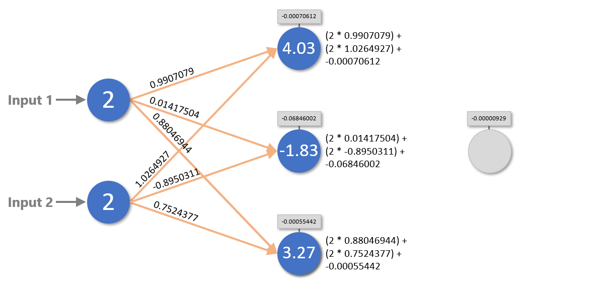
Values are propagated from the hidden layer to the output layer the same way, with one exception: they are transformed by the activation function before they’re multiplied by weights. Remember that the ReLU activation function turns negative numbers into 0s. In the example below, the -1.83 calculated for the middle neuron in the hidden layer is converted to 0, effectively eliminating that neuron’s contribution to the output.

Given a set of weights and biases, it isn’t difficult to code a neural network by hand. The following Python code models the network above:
# Weights
wac = 0.9907079
wad = 0.01417504
wae = 0.88046944

wbc = 1.0264927
wbd = -0.8950311
wbe = 0.7524377

wcf = 0.794296
wdf = 1.1687347
wef = 0.2406084

# Biases
bc = -0.00070612
bd = -0.06846002
be = -0.00055442
bf = -0.00000929

def relu(x):
    return max(0, x)

def run(a, b):
    c = (a * wac) + (b * wbc) + bc
    d = (a * wad) + (b * wbd) + bd
    e = (a * wae) + (b * wbe) + be
    f = (relu(c) * wcf) + (relu(d) * wdf) + (relu(e) * wef) + bf
    return f
If you’d like to see for yourself, paste the code into a Jupyter notebook and call the run function with the inputs 2 and 2. The answer should be very close to the actual sum of 2 and 2.
For a given problem, there is an infinite combination of weights and biases that produces the desired outcome. Here is the same network with a completely different set of weights and biases. Yet if you plug the values into the code above (or propagate values through the network by hand), you’ll find that the network is equally capable of adding 2 and 2 – or other small values, for that matter.
Once a neural network is trained, using it to make predictions is simplicity itself. It’s little more than multiplication and addition. But how do you arrive at a set of weights and biases to begin with? That’s why neural networks have to be trained.
Training Neural Networks
Training a conventional machine-learning model fits it to a dataset. Neural networks require training, too, and it is during training that weights and biases are calculated. Weights are typically initialized with small random numbers. Biases are usually initialized with 0s. In its untrained state, a neural network can’t do much more than generate random outputs. But once training is complete, the weights and biases enable the network to distinguish dogs from cats, score a book review for sentiment, or do whatever it was designed to do.
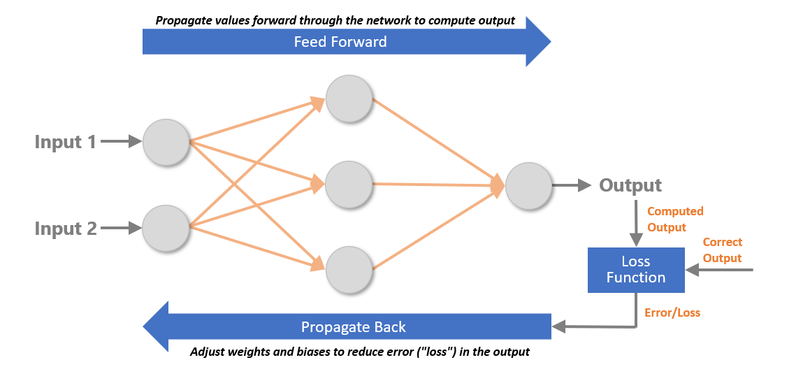
What happens when a neural network is trained? At a high level, training samples are fed through the network, the error (the difference between the computed output and the correct output) is computed using a loss function, and a backpropagation algorithm goes backward through the network adjusting the weights and biases. This is done repeatedly until the error is sufficiently small. With each iteration, the weights and biases become incrementally more refined and the error commensurately smaller.
The most critical component of the backpropagation regimen is the optimizer, which on each backward pass through the network decides how much and which direction, positive or negative, to adjust the weights and biases. Data scientists are constantly working to find better and more efficient optimizers to train networks more accurately and in less time.
Do a search on “neural networks” and you’ll turn up lots of articles with lots of complex math. Most of the math is related to optimization. An optimizer can’t just guess how to adjust the weights and biases. A neural network containing two hidden layers with 1,000 neurons each has 1,000,000 connections between layers, and therefore 1,000,000 weights to adjust. Training would take forever if the optimization strategy were simply random guessing. An optimizer must be intelligent enough to make adjustments that reduce the error in each successive iteration.
Data scientists use plots like the one below to visualize what optimizers do. The plot is called a loss landscape. It has been reduced to three dimensions for visualization purposes, but in reality, it contains many dimensions – sometimes millions of them. The multicolored contour charts the error for different combinations of weights and biases. The optimizer’s goal is to navigate the contour and find the combination that produces the least error, which corresponds to the lowest point, or global minimum, in the loss landscape.
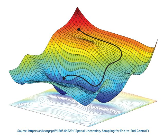
The optimizer’s job isn’t an easy one. It involves first derivatives (calculating the slope of the contour), gradient descent (adjusting weights and biases to go down the slope rather than up it or sideways), and learning rates, or how much to adjust the weights and biases in each iteration. If the learning rate is too great, the optimizer could miss the global minimum. Too small, and the network will take a long time to train. Modern optimizers use adaptive learning rates that take bigger steps when far away from a minimum and smaller steps as they approach a minimum (as the slope approaches 0). To further complicate matters, the optimizer must avoid getting trapped in local minima so it can continue traversing the contour toward the global minimum where the error is the smallest.
Neural networks are fundamentally simple. Training them is mathematically complex. Fortunately, you don’t have to understand everything that happens during training in order to build them. Deep-learning libraries such as Keras and TensorFlow insulate you from the math and provide cutting-edge optimizers that do the heavy lifting. But now when you use one of these libraries and it asks you to pick a loss function and an optimizer, you’ll understand what it’s asking for and why.
The Road Ahead
In my next post, we’ll build our first neural network. We’ll do it in Python, and we’ll see first-hand some of the decisions that go into building and training a network. It’s the next step on the journey to deep-learning enlightenment, and our first touch with what most of the world considers real AI.
