In this post, we’ll look at what linear regression is and how to create a simple linear regression machine learning model in scikit-learn.
If you want to jump straight to the code, the Jupyter notebook is on GitHub.
What is Linear Regression?
Do you remember this linear formula from algebra in school?
y=mx+b
This is the formula for a line and is the exact formula we’ll create when we make our model, but our model will fill in the m (slope) and the b (intercept) variables. We’re going to concentrate on the simple linear regression in this post, so there will only be one coefficient in our model – m.
Exploratory Data Analysis
We can’t just randomly apply the linear regression algorithm to our data. We have to make sure it’s a good fit. For this, we have to do some data analysis. But first, the ever important importing and loading of data. Thanks again to Super DataScience for openly providing datasets for public use.
import pandas as pd
import numpy as np
import matplotlib.pyplot as plt
import seaborn as sns
import statsmodels.api as sm
from sklearn.model_selection import train_test_split
from sklearn.linear_model import LinearRegression
from sklearn.metrics import r2_score

sns.set()
%matplotlib inline

df = pd.read_csv("./SalaryData.csv")
We can take a quick peek at the shape of our data.
df.shape

The data is simple and not very realistic, but it’s great for what we intend to demonstrate. Before we continue with anything else, we should check for any missing data.
df.isnull().values.any()

Awesome! No missing data. Let’s enjoy it while we can.
Splitting Data
Before we start exploring our data, we should split it up into two different data frames to work with.
Why do we need to split our data in the first place? The short answer is to take a small set of our data so we can test our model and see how well it performs on data that it hasn’t “seen” yet. Also, we need to split our features (columns our model will use to learn from) from our label (the column that has the answer we want to predict from our model).
The long answer is to prevent overfitting. Overfitting will result in a bad model. A related issue to overfitting is underfitting. Let’s go over both terms in more detail as they can be common errors in creating machine learning models and it’s important to understand them.
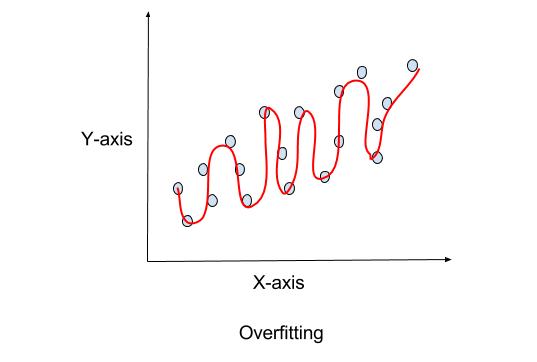
Overfitting
Overfitting a model will result in the model predicting perfect results with the training data, but once real data is provided it will generate inaccurate results compared to what the actual value should be. The plot below is a great example of it. The overfitted model is the line that goes through all points exactly. Overfitting a model won’t generalize to data that it has not seen before which will produce an inaccurate prediction.
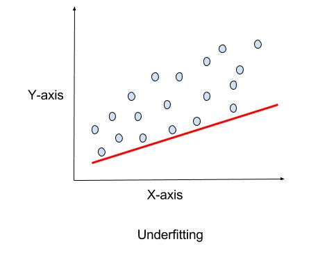
Underfitting
Underfitting is the opposite, where the model doesn’t perform very well on the training data. This usually is caused by not having enough data for the algorithm to find a pattern. Underfitting will result in the model being too simple for the data, which will result in poor performance of the model.
Splitting our Data
Now that we can see why we should split our data, let’s do it. scikit-learn provides a very helpful method for us to do just that:train_test_split
train_set, test_set = train_test_split(df, test_size=0.2, random_state=42)
In this method, we include our data frame and a test size which splits the data as 20% for our test set and 80% for our training set. A test size with an 80-20 split is common, as well as a 70-30 split. We also give the method an optional parameter for the random state. This is mainly for reproducible results as it will always split the data the same way. The method returns a tuple that we can save as our training data and our test data.
Another best practice to get in the habit of is to make a copy of your training set. This is because, as you do your exploratory data analysis, the training data can get in an unusable state to help build models. Having a copy of your training data allows you to easily and reliably reset your data analysis process.
df_copy = train_set.copy()
Exploratory Data Analysis
Now we can start the fun stuff and do some analysis. My personal preference is to start with some descriptive statistics to help me get a sense of what my data looks like.
df_copy.describe()

The average years of experience is just over five years and the average salary is $74,000.
pandas comes with a useful function for finding correlations between each of the columns.
df_copy.corr()

The years of experience and salary are positively correlated by 98%. In fact, if we plot this we can see that correlation.
df_copy.plot.scatter(x='YearsExperience', y='Salary')

That definitely looks very linear. To get an idea of what that may look like seaborn can make a line of best fit for us to visualize things.
# Regression plot
sns.regplot('YearsExperience', # Horizontal axis
           'Salary', # Vertical axis
           data=df_copy)

Looks like a great fit. Now let’s make this line ourselves by building our model.
Building the Model
In order to build our model, we need to make some changes to our training set – we have to migrate our label column to its own data frame. Our label column, or as I like to refer to the answer column, is the column that we want to predict when we run our model. I’m also going to create a copy of the test set just in case.
train_set_full = train_set.copy()

train_set = train_set.drop(["Salary"], axis=1)
Next, we’ll make a data frame of just our labels. To create this data frame, we pull the “Salary” series from the copy:
train_labels = df_copy["Salary"]
Now we can create our model with our training data.
lin_reg = LinearRegression()

lin_reg.fit(train_set, train_labels)
Here we create a new instance of the LinearRegression class and on that instance call the fit method with two parameters:
train_setis the data frame which would have the inputs – the number of years of experience.train_labelsis the series (data frame with one column) that has our answers to the input – the salary amount for specified years of experience.
And now we actually have our model. The lin_reg object can tell us more about it. For coefficients, we call the coef_ attribute, and for our intercept, we can call the intercept_ attribute:
print("Coefficients: ", lin_reg.coef_)
print("Intercept: ", lin_reg.intercept_)

We can use this information to make our model formula if we need it.
y=9423.81532303x+25321.580118
What our model tells us is that for no years of experience we should get a starting salary of $9,423.82 in salary.
To get a prediction from an input, we need to call the predict function. We can pass in a pandas series object to return an array of prediction values.
salary_pred = lin_reg.predict(test_set)

salary_pred

Or we can pass in a single value.
salary_pred = lin_reg.predict(10)

salary_pred

Scoring our Model
Now that we have our model, how do we know that it’s a good one? Or that it can work with data not in our training set? This is where the test set that we created earlier comes in.
There are a few things we can do to verify or score our model to see how well it can perform. A simple way is to compare the predicted values from the model to the actual values from our test data.
print(salary_pred)
print(test_set_full["Salary"])

The top array is our predictions and the bottom series is our actual values. Looks quite close!
There are also a couple of statistical tests we can do that come with scikit-learn that we can run. First, there’s a score method we can call directly from our model and give it our test set and test labels as parameters.
lin_reg.score(test_set, test_set_full["Salary"])

This calculates the coefficient of determination or the r^2 of the model. This can give a score between -1 and 1. Scores closer to -1 giving a negative impact on the model and scores closer to 1 give a positive impact to the model. In our case, we have 0.90 which is close to 1 which indicates that we have a pretty good model.
Be mindful when using the score method of a model. Depending on the model you execute the score method against, the type of calculation can vary. For example, the LogisticRegression class calculates the score method differently by using the accuracy score.
In that case, and we still want to get the r² of our model, we can call the r2_score method in scikit-learn. Since it does the same as our score method, we should get the same result.
r2_score(test_set_full["Salary"], salary_pred)

Our model scored a 90% for accuracy without any optimization, that is very lucky! We can take this further and see how our model plots against our test data.
plt.scatter(test_set_full["YearsExperience"], test_set_full["Salary"],  color='blue')
plt.plot(test_set_full["YearsExperience"], salary_pred, color='red', linewidth=2)

Now, that looks like a nice fit for our test data.
We built our model and were able to verify the accuracy using scoring functions. I hope this quick tutorial gave a better understanding of creating a simple linear regression model using scikit-learn. There are a ton more models to use with scikit-learn and we will have more resources to come for those
