If you’ve done even a short amount of research into data science, there is no doubt you’ve come across the Python vs. R debate. While we won’t get into which is better, there is nothing wrong with knowing both. You may be stronger in one than the other, and even prefer that one, but knowing the other language helps when reading other blog posts that go over other data science subjects.
With that in mind, let’s turn our attention away from Python for a moment and look at R. R is a language that is focused more on the statistical analysis side of computation. While it’s a bit of a niche language, it still offers a lot. In this post, we’ll go over the basics of using R with Visual Studio and what all it has to offer.
Installing R for Visual Studio
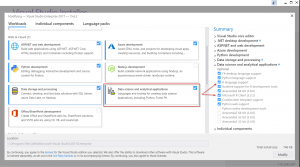
While RStudio is a great IDE for R programming, I’ll be using Visual Studio for this post. If you don’t have Visual Studio installed, feel free to head to their site and download the Community Edition. After installation, you’ll be shown the Visual Studio Installer to customize what pieces Visual Studio supports that you can install on top of it. Scroll down a bit until you see the “Data Science and analytical applications” section and make sure you check “R language support”. Feel free to include “Microsoft R client” as well. We’ll go over that in a later post. Click “Modify/install” to include it in Visual Studio.
R Interactive
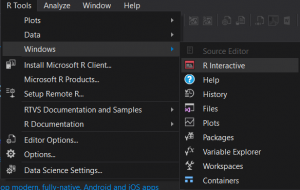
R, like Python, is a dynamic language. This means that it doesn’t have to be compiled before it runs. R includes a REPL in which you can explore code in the R Interactive. Once R is installed in Visual Studio, the RInteractive (called the “R Console” in RStudio) can be found in the top menu. When installing R you get an “R Tools” menu item. In there go to the Windows section and you can select “R Interactive”
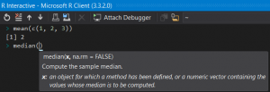
The R Interactive is powerful in itself since it offers full IntelliSense support so you can prototype and play around with aspects of the R language instantly.
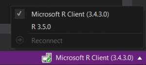
One thing to be mindful of is that you may notice that the R Interactive is using Microsoft R Client. For the most part, you won’t notice any differences between using that and a regular version of R, but some nuances exist. If you want to use the regular version and you already have it installed you can go to the bottom right of Visual Studio and select it.
Data Types
Like all other programming languages, R has their own data types. Though, as we’ll see, the biggest differences between R data types and data types from other languages are merely just in what they are called and how they are instantiated.
There are the typical types such as double for numbers and character for strings.
> typeof(2)
[1] "double"

> typeof("hello")
[1] "character"
Logical
Logical types are boolean types in R. They can be either true or false. In R, though, the syntax of these types are in all caps.
> typeof(TRUE)
[1] "logical"

> typeof(FALSE)
[1] "logical"
Logical types can be shorted to just “T” or “F”, but be mindful that it may reduce the readability of your code.
> typeof(T)
[1] "logical"

> typeof(F)
[1] "logical"
And like boolean types in other languages they can be used for comparison. To compare in R, the following operations are used:
==for equality!=for inequality>for greater than<for less than>=for greater than or equal to<=for less than or equal to
TRUE == TRUE
[1] TRUE1 == 2
[1] FALSE“test” != “TEST”
[1] TRUE1 > 1
[1] FALSE1 < 2
[1] TRUE1 >= 1
[1] TRUE1 <= 2
[1] TRUE
Like other languages, R has logical operators that you may be familiar with: && for AND and || for OR.
> 1 == 1 && 2 == 2
[1] TRUE

> 1 == 1 || 2 == 3
[1] TRUE
Vector
A vector in R is similar to other languages array type (or the list type in Python). This can hold many values of single type into a single variable. A vector can also be viewed as a one-dimensional matrix.
Vectors in R are created by using a c and enclosing elements into parentheses. If you’re wondering what the c stands for, think of it as it combining two or more types together into one.
> c(1, 2, 3)
[1] 1 2 3

> c("one", "two", "three")
[1] "one"   "two"   "three"
Viewing the type of a vector will give you the type of the items in the vector.
> typeof(c(1, 2, 3))
[1] "double"

> typeof(c("one", "two", "three"))
[1] "character"
Matrix
The matrix data type is simply a 2D vector that is in a rectangular layout. Think of a matrix as a two dimensional array in other languages.
> matrix(c(1, 2, 3))
     [,1]
[1,]    1
[2,]    2
[3,]    3
The number of rows and columns can be specified when creating a matrix into the shape that is needed.
> matrix(c(1, 2, 3, 4), nrow = 2, ncol = 2)
     [,1] [,2]
[1,]    1    3
[2,]    2    4
The byrow parameter tells the data to populate the matrix by rows first then by columns.
> matrix(c(1, 2, 3, 4), nrow = 2, ncol = 2, byrow = TRUE)
     [,1] [,2]
[1,]    1    2
[2,]    3    4
Data Frame
If you are used to Python’s pandas framework then you have R’s data frame type to thank since the creator wanted the same type of functionality within Python. Data frames are essentially a representation of tabular data. You can also think of the data looking like you would see it on a spreadsheet since it will have rows and columns with, usually, a header.
> data.frame(x = c(1, 2, 3, 4, 5), y=c(2, 4, 6, 8, 10))
  x  y
1 1  2
2 2  4
3 3  6
4 4  8
5 5 10
In the code above, we’re creating a data frame with columns x and y with data. R prints this out in a nice tabular form so that we can easily read it.
> data.frame(x = c(1, 2, 3), y=c("Yes", "No", "Maybe"))
  x     y
1 1   Yes
2 2    No
3 3 Maybe
Data frames aren’t restricted to what type each column has. Above we specified the x column as numbers but the y column has strings.
Factor
Factors in R are a special string type that supports categories. While you can support categories as a vector of strings, the factor type gives some extra support for categorical data.
> items = c("Yes", "No", "No", "Yes", "Yes")
> items
[1] "Yes" "No"  "No"  "Yes" "Yes"
> factor(items)
[1] Yes No  No  Yes Yes
Levels: No Yes
Notice the “Levels” in the output when converting a vector into a factor. That just indicates which unique items are in the category. If we need we can get the levels themselves.
> levels(factor(items))
[1] "No"  "Yes"
Some categorical values can be ordinal, or that they have a specific order to them. For example, suppose that we have a categorical column that has categories such as “
Formulas
With R being a statistical programming language it has some nuances in it that help programmers express mathematical models much easier. With that comes the formula type. This type uses the ~ (tilde) symbol and can look confusing at first.
An Aside On Sample Data
Before we get into formulas, we would need some data to use it on. As an example, say we want to look at data on cars. R has some built in data sets that we can play around with using the data() function. Using it without any parameters brings up a list of available data sets.
> data()
Data sets in package ‘datasets’:

AirPassengers           Monthly Airline Passenger Numbers 1949-1960
BJsales                 Sales Data with Leading Indicator
BJsales.lead (BJsales)
                        Sales Data with Leading Indicator
BOD                     Biochemical Oxygen Demand
CO2                     Carbon Dioxide Uptake in Grass Plants
ChickWeight             Weight versus age of chicks on different diets
DNase                   Elisa assay of DNase
EuStockMarkets          Daily Closing Prices of Major European Stock
                        Indices, 1991-1998
To load any of them, add the name of the data set you want as a parameter, without making it a string. I’ll be using the mtcars dataset as an example.
> data(mtcars)
> mtcars
                     mpg cyl  disp  hp drat    wt  qsec vs am gear carb
Mazda RX4           21.0   6 160.0 110 3.90 2.620 16.46  0  1    4    4
Mazda RX4 Wag       21.0   6 160.0 110 3.90 2.875 17.02  0  1    4    4
Datsun 710          22.8   4 108.0  93 3.85 2.320 18.61  1  1    4    1
Hornet 4 Drive      21.4   6 258.0 110 3.08 3.215 19.44  1  0    3    1
Hornet Sportabout   18.7   8 360.0 175 3.15 3.440 17.02  0  0    3    2
Valiant             18.1   6 225.0 105 2.76 3.460 20.22  1  0    3    1
You can also find more information about the data set by putting a question mark (?) in front of the name.

And Now Back to Formulas
With our data now loaded, we can use it in a formula.
> formula = as.formula(mpg ~ cyl + disp)

> typeof(formula)
[1] "language"
> class(formula)
[1] "formula"
The as.formula is a function in R. You can think of any of the as. functions as being able to parse from one data type to another. You’ll notice in R that function names have dots in them. Personally, that seems confusing so I tend to avoid that when creating functions.
The best way to describe what the formula is doing is that we’re indicating to R that mpg is a function of cyl and disp. Or, a way I like to look at it, is that we’re telling R that mpg = cyl + disp. Formulas will take some time to get used to, but with practice, you’ll get the hang of using them and even begin to appreciate it.
In this post, we went over how you can use R in Visual Studio and went over the basic data types you will be using within your R journey into data science. I hope this whets your appetite for more R because, in our next post for R programming, we’ll go over how to use programming paradigms in R.
